Consistent with the findings of Granger and Ding (1996), informal investigations reveal that the dynamic dependencies are significantly more pronounced for the absolute as opposed to the squared sample returns. Consequently, our intraday modeling focuses on the patterns in \Rt\ and \R, , rather than R1, and Я2 .

interdaily return autocorrelations, without affecting the autocorrelation pattern 21. In contrast, the periodicity may have a strong impact on the autocorrelation pattern for the absolute intraday returns. Straightforward calculations reveal

Corr(tf,J,\RTJ)

M(ssn m)Cow(at, <rr) +Cov(s , s,n)E2(a,) M(V)Var(cr() +cNE(a,2)M(s2) + £2( tr,)Var( s)

where VaKs) s M(s2) - М2(Д Cov(sn, sm) = M(ssnm) - M2(s) and cN = E~2\Ztn\ - 1. Eq. (4) illustrates the interaction between the periodicity in absolute returns at the intradaily level and the conditional heteroskedasticity at the daily level. For adjacent trading days the impact of the positive correlation in the daily return volatility, captured by Cov(ot, aT), is strong and induces positive dependence in the absolute returns, but as the distance between t and т grows this effect becomes less important which is consistent with the slow decay in the correlo-grams in the bottom panels of Fig. 4. At the same time, the correlograms are affected by the strong intraday periodicity. For example, consider the display for the absolute S&P 500 returns in Fig. 4b. The correlations attain their lowest values around lag forty, or half a trading day. This corresponds to the bottom of the U-shape for the average absolute returns depicted in Fig. 2b. Clearly, the population covariance, Cov(sn, sm), is minimized and significantly negative, at this frequency. Eq. (4) verifies that the negative correlation between the 5-minute absolute returns, realized about half-a-day apart, translates into a negative contribution to the corresponding correlogram at the 3-4 hour frequencies. Likewise, Fig. 2a indicates that there is strong negative correlation between the absolute foreign exchange returns in the intervals 80-225 (covering about half-a-day) and all the remaining 5-minute returns. Not surprisingly, the lower panel of Fig. 4a verifies that this again results in highly significant troughs in the correlogram around the 12 hour frequency (and its harmonics). Indeed, the impact is now sufficiently strong that the absolute return autocorrelations turn negative. This is truly remarkable given the very large positive autocorrelations found at the daily frequency and it is testimony to the profound impact of the periodic structure on the intraday return dynamics. In terms of the specification in Eq. (4), the size of the second, negative, term of the numerator exceeds the first, positive, term around the 12 hour frequency.

3.3. Long-run implications and comparison to daily returns

To further assess the descriptive accuracy of the formulation in Eq. (1), we now investigate the long-run implications for the correlogram. It is convenient to focus on the daily frequency i.e. n = m,

Corr(J?li(I, \RTJ)

Cov(cr(, cr) + (Vht(s)/M(s2))E2(o-,) Var(a,) + cNE(a2) + (Var(s)/M(s2))E2(a,)

Fig. 5a and b display the first forty autocorrelations for the absolute returns of the two daily time series on the DM-$ spot exchange rate and the S&P 500 cash

(а) -г

-0.10

(b) 020

0.15

-0.10

0 4

0 4

Dally. Rt - Five-Minute, Rn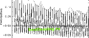

12 16 20 24 28 32 36 40 Daily Lag

Daily. Rt FiTe-Minute, Rt1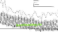

12 16 20 24 28 32 36 40 Daily Lag

Fig. 5. Forty days correlogram of absolute returns, (a) DM-$, (b) S&P 500.

4. Implications for volatility modeling and high frequency return aggregation

Section 3 demonstrates that the distinct intraday periodicity has a strong impact on the autocorrelation patterns of the 5-minute returns. The question therefore arises whether more formal time series modeling of return volatility is similarly affected by the presence of periodic features, and if so, whether some observation intervals are preferable relative to others for the purpose of drawing inference concerning the dynamic features of interest. In order to address these issues this section presents an extensive analysis of the properties of the return series obtained at a range of different intradaily and interdaily frequencies.

4.1. Characterization of the intraday returns at the various frequencies

Summary statistics for the foreign exchange market are provided in Table la for all seventeen possible intraday returns with a 24-hour periodicity. The returns are continuously compounded i.e. the wth return on day t for the series at (k 5)-minute intervals is defined by Rkt = £, = ( \)k+],nktj t= 1,2, ..., 260,

The sample autocorrelations are generally negatively biased and become less precise as the lag length grows; see Percival (1993) who point out that the sum of all the sample autocorrelations by construction equals zero. We therefore limit our analysis to lag-lengths which may appear large, but nonetheless constitute a modest fraction of the total intraday sample.

23 The slow rate of decay in the autocorrelation functions is also in accordance with the apparent long-memory feature of asset return volatility documented by a number of recent studies (see e.g. Baillie et al., 1996; Ding et al., 1993).

index, along with the corresponding 5-minute intraday autocorrelations out to lag 11,520 and 3,200, respectively 22. Direct comparison between the empirically estimated Corr(l l#Tl) in Eq. (3) and the expression for Corr(/? L \RT<n\) above are complicated by the different sample periods required for reliable inference. Nonetheless, it is clear that the decay rate in the local maxima of the intradaily absolute correlogram and the daily return autocorrelations should be qualitatively comparable, as the Cov(tr aT) term governs both. Comparing the peaks in the intraday correlograms to the daily autocorrelations in Fig. 5a and b confirms this implication of our stylized model; the dominant rate of decay is strikingly similar for both markets 23.

The findings in this section demonstrate a strong correspondence between the qualitative implications of the model outlined in Eq. (1) and the stylized empirical facts. It suggests that our model, stressing the conditional heteroskedasticity at the daily level along with the strong deterministic periodicity at the intradaily level, may serve as a good starting point for high frequency volatility modeling and as such it constitutes the basis for the subsequent analysis in Section 5.