lagged squared innovation, (e,*,)2, relative to the overall volatility level, (o;kn i)2, hence explaining the relatively large estimates for a(k) at the shortest return intervals. For the intermediate hour return models the change in the

average volatility between sampling intervals will typically appear much more abrupt, resulting in significantly lower persistence measures. Beyond the 2-hour intervals the periodic pattern is averaged over a substantial part of the 24-hour trading day, and the intraday exchange rate estimates are generally closer to the implications obtained from daily models.

The results for the S&P 500 equity returns tell a similar story. The interdaily estimates in Table 3b are again broadly consistent with the a priori predictions based on the daily GARCH(1, 1) model 33. Although the volatility persistence is higher than for the foreign exchange returns, a{k) + [3lk) again displays a general smooth decline and the explicit persistence measures are fairly stable across the different return horizons. The discrepancy between the half lives, mean lags and median lags implied by the intradaily and interdaily returns are even stronger than for the foreign exchange rate data, however 34. Moreover, the pattern in the intraday estimates for a(lt) + (5(k) reported in Table 2b is again erratic, reaching lows at the {-day (k = 40) and 20-25 minute (k = 4, 5) return horizons, and highs at the 40-50 minute (k = 8, 10) and 5-minute (k = 1) horizons. We conclude that the daily GARCH models conform closely to the theoretical predictions, but the strong intraday periodic patterns in volatility render the intradaily estimates highly variable and generally hard to interpret.

5. The dynamics of filtered and standardized intraday returns

This section proposes a general framework for modeling of high frequency return volatility that explicitly incorporates the effect of the intraday periodicity. The preceding section suggests that this is a prerequisite for meaningful time series analysis. Our approach is motivated by the stylized model in Section 3. While the model almost certainly is overly simplistic, the previous analysis suggests that the representation does capture the dominant features of our foreign exchange and equity return series and thus may serve as a reasonable first approximation.

3 In this case the estimate for the daily MA(1) term equals 0.186, which is highly significant when judged by the corresponding asymptotic standard error of 0.012. Consequently the GARCHO, 1) models for the other frequencies are, at best, approximate representations of the data generating process (see Drost and Nijman (1993) for a formal analysis).

34 The previous footnote about the deletion of weekend exchange rate returns are even more pertinent here as both weekend and overnight equity returns are excluded. However, our informal analysis again found this to be inconsequential (see Andersen and Bollerslev, 1994).

Specifically, consider the following decomposition for the intraday returns, R n=E(Rlin) + §, (7)

where E(Rln) denotes the unconditional mean, and N refers to the number of return intervals per day. Notice that this represents a generalization of the model in Section 3, in that the periodic component for the nth intraday interval, s, n, is allowed to depend on the characteristics of trading day, t 35. Given the absence of any economic theory for stipulating a particular parametric form for the intraday periodic structure, a flexible nonparametric procedure seems natural. Although no one procedure is clearly superior, the smooth cyclical patterns documented in Fig. 2a and b naturally lend themselves to estimation by the Fourier flexible functional form introduced by Gallant, 1981, 1982 36. In a related context, Dacorogna et al. (1993) have proposed estimating the periodicity in the activity in the foreign exchange market as the sum of three polynomials corresponding to the distinct geographical locations of the market. Returns measured on their resulting theta-time scale correspond closely to our filtered returns defined and analyzed below. However, one advantage of the approach advocated here is that it allows the shape of the periodic pattern in the market to also depend on the overall level of the volatility; a feature which turns out to be important for the equity market. Also, the combination of trigonometric functions and polynomial terms are likely to result in better approximation properties when estimating regularly recurring patterns. Furthermore, our approach for estimating st n utilizes the full time series dimension of the returns data, as opposed to simply estimating the average pattern across the trading day. Full details of the approach are provided in Appendix B. Meanwhile, it is clear from the estimated average intraday periodic patterns depicted in Fig. 6a and b, that the fitted values, stn, provide a close approximation to the overall volatility patterns in both markets. Of course, the usefulness of the procedure will ultimately depend upon the degree to which it is successful in identifying the periodic components in a temporal dimension as well. If so, the approach may serve as the basis for a nonlinear filtering procedure that could eliminate the periodic components prior to the analysis of any intraday return volatility dynamics 37.

This feature is particularly important for the equity returns for which the general U-shaped volatility pattern is transformed into more of a J-shape on the highest volatility days (see Andersen and Bollerslev, 1994).

36 This technique has previously been applied to financial return series in a different context by Pagan and Schwert (1990).

37 This same methodology may also be used directly for prediction of future volatility over different intraday time intervals. Such intraday volatility prediction may be particularly important in the pricing and/or continuous re-balancing of hedged intraday options positions. We shall not pursue this issue any further here, however.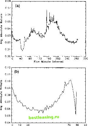

30 40 50 60 Five Minute Interval

Fig. 6. Flexible Fourier functional form of intraday average absolute returns, (a) DM-$, (b) S&P 500. 5.1. Filtered foreign exchange returns

To further investigate these issues, define the filtered 5-minute return series; R, n = Rtn/st n 38. If the characterization of the 5-minute return series in Eq. (7) is perfect and the associated estimation error is negligible, then ignoring the impact of the weak first order return correlation, the filtered returns should conform more closely to the theoretical aggregation results for the GARCHG, 1) model. We explicitly consider how well this hypothesis holds up, but we also keep in mind

38 Alternatively, Rt might also be mean adjusted. Since the mean return is practically zero, this is immaterial.