Unlike the traditional clothing size systems, the one Ashdown and Paal came up with is not an ordered set of graduated sizes where all dimensions increase together. Instead, they came up with sizes that fit particular body types. Each body type corresponds to a cluster of records in a database of body measurements. One cluster might consist of short-legged, small-waisted, large-busted women with long torsos, average arms, broad shoulders, and skinny necks while other clusters capture other constellations of measurements.

The database contained more than 100 measurements for each of nearly 3,000 women. The clustering technique employed was the K-means algorithm, described in the next section. In the end, only a handful of the more than 100 measurements were needed to characterize the clusters. Finding this smaller number of variables was another benefit of the clustering process.

K-Means Clustering

The K-means algorithm is one of the most commonly used clustering algorithms. The K in its name refers to the fact that the algorithm looks for a fixed number of clusters which are defined in terms of proximity of data points to each other. The version described here was first published by J. B. MacQueen in 1967. For ease of explaining, the technique is illustrated using two-dimensional diagrams. Bear in mind that in practice the algorithm is usually handling many more than two independent variables. This means that instead of points corresponding to two-element vectors (xi,x2), the points correspond to n-element vectors (x!,x2, . . . , xn). The procedure itself is unchanged.

Three Steps of the K-Means Algorithm

In the first step, the algorithm randomly selects K data points to be the seeds. MacQueens algorithm simply takes the first K records. In cases where the records have some meaningful order, it may be desirable to choose widely spaced records, or a random selection of records. Each of the seeds is an embryonic cluster with only one element. This example sets the number of clusters to 3.

The second step assigns each record to the closest seed. One way to do this is by finding the boundaries between the clusters, as shown geometrically in Figure 11.3. The boundaries between two clusters are the points that are equally close to each cluster. Recalling a lesson from high-school geometry makes this less difficult than it sounds: given any two points, A and B, all points that are equidistant from A and B fall along a line (called the perpendicular bisector) that is perpendicular to the one connecting A and B and halfway between them. In Figure 11.3, dashed lines connect the initial seeds; the resulting cluster boundaries shown with solid lines are at right angles to

the dashed lines. Using these lines as guides, it is obvious which records are closest to which seeds. In three dimensions, these boundaries would be planes and in N dimensions they would be hyperplanes of dimension N - 1. Fortunately, computer algorithms easily handle these situations. Finding the actual boundaries between clusters is useful for showing the process geometrically. In practice, though, the algorithm usually measures the distance of each record to each seed and chooses the minimum distance for this step.

For example, consider the record with the box drawn around it. On the basis of the initial seeds, this record is assigned to the cluster controlled by seed number 2 because it is closer to that seed than to either of the other two.

At this point, every point has been assigned to exactly one of the three clusters centered around the original seeds. The third step is to calculate the cen-troids of the clusters; these now do a better job of characterizing the clusters than the initial seeds Finding the centroids is simply a matter of taking the average value of each dimension for all the records in the cluster.

In Figure 11.4, the new centroids are marked with a cross. The arrows show the motion from the position of the original seeds to the new centroids of the clusters formed from those seeds.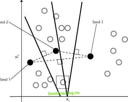

Figure 11.3 The initial seeds determine the initial cluster boundaries.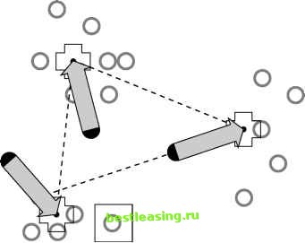

Figure 11.4 The centroids are calculated from the points that are assigned to each cluster.

The centroids become the seeds for the next iteration of the algorithm. Step 2 is repeated, and each point is once again assigned to the cluster with the closest centroid. Figure 11.5 shows the new cluster boundaries-formed, as before, by drawing lines equidistant between each pair of centroids. Notice that the point with the box around it, which was originally assigned to cluster number 2, has now been assigned to cluster number 1. The process of assigning points to cluster and then recalculating centroids continues until the cluster boundaries stop changing. In practice, the K-means algorithm usually finds a set of stable clusters after a few dozen iterations.

What K Means

Clusters describe underlying structure in data. However, there is no one right description of that structure. For instance, someone not from New York City may think that the whole city is downtown. Someone from Brooklyn or Queens might apply this nomenclature to Manhattan. Within Manhattan, it might only be neighborhoods south of 23rd Street. And even there, downtown might still be reserved only for the taller buildings at the southern tip of the island. There is a similar problem with clustering; structures in data exist at many different levels.