Gaussian mixture models are a probabilistic variant of K-means. The name comes from the Gaussian distribution, a probability distribution often assumed for high-dimensional problems. The Gaussian distribution generalizes the normal distribution to more than one variable. As before, the algorithm starts by choosing K seeds. This time, however, the seeds are considered to be the means of Gaussian distributions. The algorithm proceeds by iterating over two steps called the estimation step and the maximization step.

The estimation step calculates the responsibility that each Gaussian has for each data point (see Figure 11.8). Each Gaussian has strong responsibility for points that are close to its mean and weak responsibility for points that are distant. The responsibilities are be used as weights in the next step.

In the maximization step, a new centroid is calculated for each cluster taking into account the newly calculated responsibilities. The centroid for a given Gaussian is calculated by averaging all the points weighted by the responsibilities for that Gaussian, as illustrated in Figure 11.9.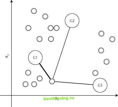

Figure 11.8 In the estimation step, each Gaussian is assigned some responsibility for each point. Thicker lines indicate greater responsibility.

These steps are repeated until the Gaussians no longer move. The Gaussians themselves can change in shape as well as move. However, each Gaussian is constrained, so if it shows a very high responsibility for points close to its mean, then there is a sharp drop off in responsibilities. If the Gaussian covers a larger range of values, then it has smaller responsibilities for nearby points. Since the distribution must always integrate to one, Gaussians always gets weaker as they get bigger.

The reason this is called a mixture model is that the probability at each data point is the sum of a mixture of several distributions. At the end of the process, each point is tied to the various clusters with higher or lower probability. This is sometimes called soft clustering, because points are not uniquely identified with a single cluster.

One consequence of this method is that some points may have high probabilities of being in more than one cluster. Other points may have only very low probabilities of being in any cluster. Each point can be assigned to the cluster where its probability is highest, turning this soft clustering into hard clustering.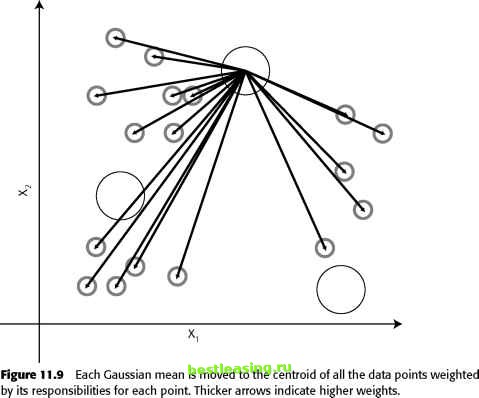

Agglomerative Clustering

The K-means approach to clustering starts out with a fixed number of clusters and allocates all records into exactly that number of clusters. Another class of methods works by agglomeration. These methods start out with each data point forming its own cluster and gradually merge them into larger and larger clusters until all points have been gathered together into one big cluster. Toward the beginning of the process, the clusters are very small and very pure-the members of each cluster are few and closely related. Towards the end of the process, the clusters are large and not as well defined. The entire history is preserved making it possible to choose the level of clustering that works best for a given application.

An Agglomerative Clustering Algorithm

The first step is to create a similarity matrix. The similarity matrix is a table of all the pair-wise distances or degrees of similarity between clusters. Initially, the similarity matrix contains the pair-wise distance between individual pairs of records. As discussed earlier, there are many measures of similarity between records, including the Euclidean distance, the angle between vectors, and the ratio of matching to nonmatching categorical fields. The issues raised by the choice of distance measures are exactly the same as those previously discussed in relation to the K-means approach.

It might seem that with N initial clusters for N data points, N2 measurement calculations are required to create the distance table. If the similarity measure is a true distance metric, only half that is needed because all true distance metrics follow the rule that Distance(X,Y) = Distance(Y,X). In the vocabulary of mathematics, the similarity matrix is lower triangular. The next step is to find the smallest value in the similarity matrix. This identifies the two clusters that are most similar to one another. Merge these two clusters into a new one and update the similarity matrix by replacing the two rows that described the parent cluster with a new row that describes the distance between the merged cluster and the remaining clusters. There are now N - 1 clusters and N - 1 rows in the similarity matrix.

Repeat the merge step N - 1 times, so all records belong to the same large cluster. Each iteration remembers which clusters were merged and the distance between them. This information is used to decide which level of clustering to make use of.

Distance between Clusters

A bit more needs to be said about how to measure distance between clusters. On the first trip through the merge step, the clusters consist of single records so the distance between clusters is the same as the distance between records, a subject that has already been covered in perhaps too much detail. Second and