subsequent trips through the loop need to update the similarity matrix with the distances from the new, multirecord cluster to all the others. How do we measure this distance?

As usual, there is a choice of approaches. Three common ones are:

Single linkage

Complete linkage

Centroid distance

In the single linkage method, the distance between two clusters is given by the distance between the closest members. This method produces clusters with the property that every member of a cluster is more closely related to at least one member of its cluster than to any point outside it.

Another approach is the complete linkage method, where the distance between two clusters is given by the distance between their most distant members. This method produces clusters with the property that all members lie within some known maximum distance of one another.

Third method is the centroid distance, where the distance between two clusters is measured between the centroids of each. The centroid of a cluster is its average element. Figure 11.10 gives a pictorial representation of these three methods.

Closest clusters by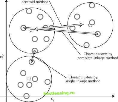

Figure 11.10 Three methods of measuring the distance between clusters.

Clusters and Trees

The agglomeration algorithm creates hierarchical clusters. At each level in the hierarchy, clusters are formed from the union of two clusters at the next level down. A good way of visualizing these clusters is as a tree. Of course, such a tree may look like the decision trees discussed in Chapter 6, but there are some important differences. The most important is that the nodes of the cluster tree do not embed rules describing why the clustering takes place; the nodes simply state the fact that the two children have the minimum distance of all possible clusters pairs. Another difference is that a decision tree is created to maximize the leaf purity of a given target variable. There is no target for the cluster tree, other than self-similarity within each cluster. Later in this chapter well discuss divisive clustering methods. These are similar to the agglomera-tive methods, except that agglomerative methods are build by starting from the leaving and working towards the root whereas divisive methods start at the root and work down to the leaves.

Clustering People by Age: An Example of Agglomerative Clustering

This illustration of agglomerative clustering uses an example in one dimension with the single linkage measure for distance between clusters. These choices make it possible to follow the algorithm through all its iterations without having to worry about calculating distances using squares and square roots.

The data consists of the ages of people at a family gathering. The goal is to cluster the participants using their age, and the metric for the distance between two people is simply the difference in their ages. The metric for the distance between two clusters of people is the difference in age between the oldest member of the younger cluster and the youngest member of the older cluster. (The one dimensional version of the single linkage measure.)

Because the distances are so easy to calculate, the example dispenses with the similarity matrix. The procedure is to sort the participants by age, then begin clustering by first merging clusters that are 1 year apart, then 2 years, and so on until there is only one big cluster.

Figure 11.11 shows the clusters after six iterations, with three clusters remaining. This is the level of clustering that seems the most useful. The algorithm appears to have clustered the population into three generations: children, parents, and grandparents.

Distance 6

Distance 5

Distance 4

Distance 3

Distance 2

Distance 1

Figure 11.11 An example of agglomerative clustering.

Divisive Clustering

We have already noted some similarities between trees formed by the agglomerative clustering techniques and ones formed by decision tree algorithms. Although the agglomerative methods work from the leaves to the root, while the decision tree algorithms work from the root to the leaves, they both create a similar hierarchical structure. The hierarchical structure reflects another similarity between the methods. Decisions made early on in the process are never revisited, which means that some fairly simple clusters may not be detected if an early split or agglomeration destroys the structure.

Seeing the similarity between the trees produced by the two methods, it is natural to ask whether the algorithms used for decision trees may also be used for clustering. The answer is yes. A decision tree algorithm starts with the entire collection of records and looks for a way to split it into partitions that are purer, in some sense defined by a purity function. In the standard decision tree algorithms, the purity function uses a separate variable-the target variable-to make this decision. All that is required to turn decision trees into a clustering