Table 12.4 From Times to Hazards

Notice in Table 12.4 that the censoring takes place one time unit later than the lifetime. That is, Customer #1 survived to Time 5, what happens after that is unknown. The hazard at a given time is the number of customers who are STOPPED divided by the total of the customers who are either ACTIVE or STOPPED. xk/P

The hazard for Time 1 is 14 percent, since one out of seven customers stop at this time. All seven customers survived to time 1 and all could have stopped. Of these, only one did. At TIME 2, there are five customers left-Customer #7 has already stopped, and Customer #6 has been censored. Of these five, one stops, for a hazard of 20 percent. And so on. This example has shown how to calculate hazard functions, taking into account the fact that some (hopefully many) customers have not yet stopped.

This calculation also shows that the hazards are highly erratic-jumping from 25 percent to 50 percent to 0 percent in the last 3 days. Typically, hazards do not vary so much. This erratic behavior arises only because there are so few customers in this simple example. Similarly, lining up customers in a table is useful for didactic purposes to demonstrate the calculation on a manageable set of data. In the real world, such a presentation is not feasible, since there are likely to be thousands or millions of customers going down and hundreds or thousands of days going across.

It is also worth mentioning that this treatment of hazards introduces them as conditional probabilities, which vary between 0 and 1. This is possible because the hazards are using time that is in discrete units, such as days or week, a description of time applicable to customer-related analyses. However, statisticians often work with hazard rates rather than probabilities. The ideas are clearly very related, but the mathematics using rates involves daunting integrals, complicated exponential functions, and difficult to explain adjustments to this or that factor. For our purposes, the simpler hazard probabilities are not only easier to explain, but they also solve the problems that arise when working with customer data.

Other Types of Censoring

The previous section introduced censoring in two cases: hazards for customers after they have stopped and hazards for customers who are still active. There

Team-Ffy®

are other useful cases as well. To explain other types of censoring, it is useful to go back to the medical realm.

Imagine that you are a cancer researcher and have found a medicine that cures cancer. You have to run a study to verify that this fabulous new treatment works. Such studies typically follow a group of patients for several years after the treatment, say 5 years. For the purposes of this example, we only want to know if patients die from cancer during the course of the study (medical researchers have other concerns as well, such as the recurrence of the disease, but that does not concern us in this simplified example).

So you identify 100 patients, give them the treatment, and their cancers seem to be cured. You follow them for several years. During this time, seven patients celebrate their newfound health by visiting Iceland. In a horrible tragedy, all seven happen to die in an avalanche caused by a submerged volcano. What is the effectiveness of your treatment on cancer mortality? Just looking at the data, it is tempting to say there is a 7 percent mortality rate. However, this mortality is clearly not related to the treatment, so the answer does not feel right.

And, in fact, the answer is not right. This is an example of competing risks. A study participant might live, might die of cancer, or might die of a mountain climbing accident on a distant island. Or the patient might move to Tahiti and drop out of the study. As medical researchers say, such a patient has been lost to follow-up.

The solution is to censor the patients who exit the study before the event being studied occurs. If patients drop out of the study, then they were healthy to the point in time when they dropped out, and the information acquired during this period can be used to calculate hazards. Afterward there is no way of knowing what happened. They are censored at the point when they exit. If a patient dies of something else, then he or she is censored at the point when death occurs, and the death is not included in the hazard calculation.

The right way to deal with competing risks is to develop different sets of hazards for each risk, where the other risks are censored.

Competing risks are familiar in the business environment as well. For instance, there are often two types of stops: voluntary stops, when a customer decides to leave, and involuntary stops, when the company decides a customer should leave-often due to unpaid bills

In doing an analysis on voluntary churn, what happens to customers who are forced to discontinue their relationships due to unpaid bills? If such a customer were forced to stop on day 100, then that customer did not stop voluntarily on days 1-99. This information can be used to generate hazards for voluntary stops. However, starting on day 100, the customer is censored, as shown in Figure 12.8. Censoring customers, even when they have stopped for other reasons, makes it possible to understand different types of stops.

These two customers were forced to leave, so they are censored at the point of attrition instead of being considered stopped.

All the data from before they left is included in the calculation of the hazard functions for voluntary attrition -since this they remained as customers before then.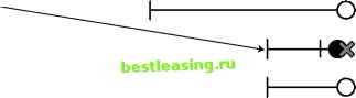

time

Figure 12.8 Using censoring makes it possible to develop hazard models for voluntary attrition that include customers who were forced to leave.

From Hazards to Survival

This chapter started with a discussion of retention curves. From the hazard functions, it is possible to create a very similar curve, called the survival curve. The survival curve is more useful and in many senses more accurate.

Retention

A retention curve provides information about how many customers have been retained for a certain amount of time. One common way of creating a retention curve is to do the following:

For customers who started 1 week ago, measure the 1-week retention.

For customers who started 2 weeks ago, measure the 2-week retention.

And so on.

Figure 12.9 shows an example of a retention curve based on this approach. The overall shape of this curve looks appropriate. However, the curve itself is quite jagged. It seems odd, for instance, that 10-week retention would be better than 9-week retention, as suggested by this data.