The first work on genetic algorithms dates back to the late 1950s, when biologists and computer scientists worked together to model the mechanisms of evolution on early computers. A bit later, in the early 1960s, Professor John Holland and his colleagues at the University of Michigan applied this work on computerized genetics-chromosomes, genes, alleles, and fitness functions- to optimization problems. In 1967, one of Hollands students, J. D. Bagley, coined the term genetic algorithms in his graduate thesis to describe the optimization technique. At the time, many researchers were uncomfortable with genetic algorithms because of their dependence on random choices during the process of evolving a solution; these choices seemed arbitrary and unpredictable. In the 1970s, Prof. Holland developed a theoretical foundation for the technique. His theory of schemata gives insight into why genetic algorithms work-and intriguingly suggests why genetics itself creates successful, adaptable creatures such as ourselves.

In the world of data mining and data analysis, the use of genetic algorithms has not been as widespread as the use of other techniques. Data mining focuses on tasks such as classification and prediction, rather than on optimization. Although many data mining problems can be framed as optimization problems, this is not the usual description. For instance, a typical data mining problem might be to predict the level of inventory needed for a given item in a catalog based on the first week of sales, characteristics about the items in the catalog, and its recipients. Rephrasing this as an optimization problem turns it into something like what function best fits the inventory curve for predictive purposes. Applying statistical regression techniques is one way to find the function. Feeding the data into a neural network is another way of estimating it. Using genetic algorithms offers another possibility. The aside Optimization discusses other methods designed specifically for this purpose.

This chapter covers the background of genetics on computers, and introduces the schema mechanism invented by John Holland to explain why genetic algorithms work. It talks about two case studies, one in the area of resource optimization and the other in the area of classifying email messages. Although few commercial data mining products include genetic algorithms (GAs), more specialized packages do support the algorithms. They are an important and active area of research and may become more widely used in the future.

How They Work

The power of genetic algorithms comes from their foundation in biology, where evolution has proven capable of adapting life to a multitude of environments (see sidebar Simple Overview of Genetics ). The success of mapping the

template for the human genome-all the common DNA shared by human individuals-is just the beginning. The human genome has been providing knowledge for advances in many fields, such as medical research, biochemistry, genetics, and even anthropology. Although interesting, human genomics is fortunately beyond the scope of knowledge needed to understand genetic algorithms. The language used to describe the computer technique borrows heavily from the biological model, as discussed in the following section.

Genetics on Computers

A simple example helps illustrate how genetic algorithms work: trying to find the maximum value of a simple function with a single integer parameter p. The function in this example is the parabola (which looks like an upside-down U ) defined by 31p - p2 where p varies between 0 and 31 (see Figure 13.1). The parameter p is expressed as a string of 5 bits to represent the numbers from 0 to 31; this bit string is the genetic material, called a genome. The fitness function peaks at the values 15 and 16, represented as 01111 and 10000, respectively. This example shows that genetic algorithms are applicable even when there are multiple, dissimilar peaks.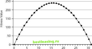

Parameter p

Figure 13.1 Finding the maximum of this simple function helps illustrate genetic algorithms.

GAs work by evolving successive generations of genomes that get progressively more and more fit; that is, they provide better solutions to the problem. In nature, fitness is simply the ability of an organism to survive and reproduce. On a computer, evolution is simulated with the following steps:

1. Identify the genome and fitness function.

2. Create an initial generation of genomes.

3. Modify the initial population by applying the operators of genetic algorithms.

4. Repeat Step 3 until the fitness of the population no longer improves.

The first step is setting up the problem. In this simple example, the genome consists of a single, 5-bit gene for the parameter p. The fitness function is the parabola. Over the course of generations, the fitness function is going to be maximized.

For this example, shown in Table 13.1, the initial generation consists of four genomes, randomly produced. A real problem would typically have a population of hundreds or thousands of genomes, but that is impractical for illustrative purposes. Notice that in this population, the average fitness is 122.5-pretty good, since the actual maximum is 240, but evolution can improve it.

The basic algorithm modifies the initial population using three operators- selection, then crossover, then mutation-as illustrated in Figure 13.2. These operators are explained in the next three sections.