Histograms, such as those in Figure 17.2, shows how often each value or range of values occurs in some set of data. The vertical axis is a count of records, and the horizontal axis is the values in the column. The shape of this histogram shows the distribution of the values (strictly speaking, in a distribution, the counts are divided by the total number of records so the area under the curve is one). If we are working with a sample, and the sample is randomly chosen, then the distribution of values in the subset should be about the same as the distribution in the original data.

This histogram is for the month of claim for a set of insurance claims.

This is an example of a typically uniform distribution. That is, the number of claims is roughly the same for each month.

June

July

Sept

This histogram shows the number of telephone calls made for different durations.

This is an example of an exponentially decreasing distribution.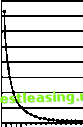

li -6- -а- б- d, <v л a 4 rv i a .i <v <v

Duration

(Minutes)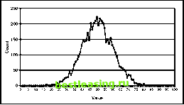

This histogram shows a normal distribution with a mean of 50 and a standard deviation of 10. Notice that high and low values are very rare.

Figure 17.2 Histograms show the distribution of data values.

The distribution of the values provides important insights into the data. It shows which values are common and which are less common. Just looking at the distribution of values brings up questions-such as why an amount is negative or why some categorical values are not present. Although statisticians tend to be more concerned with distributions than data miners, it is still important to look at variable values. Here, we illustrate some special cases of distributions that are important for data mining purposes, as well as the special case of variables synonymous with the target.

Columns with One Value

The most degenerate distribution is a column that has only one value. Unary-valued columns, as they are more formally known, do not contain any information that helps to distinguish between different rows. Because they lack any information content, they should be ignored for data mining purposes.

Having only one value is sometimes a property of the data. It is not uncommon, for instance, for a database to have fields defined in the database that are not yet populated. The fields are only placeholders for future values, so all the values are uniformly something such as null or no or 0.

Before throwing out unary variables, check that NULLs are being counted as values. Appended demographic variables sometimes have only a single value or NULL when the value is not known. For instance, if the data provider knows that someone is interested in golf-say because the person subscribes to a golfing magazine or belongs to a country club-then the golf-enthusiast flag would be set to Y. When there is no evidence, many providers set the flag to NULL-meaning unknown-rather than N.

When a variable has only one value, be sure (1) that NULL is being included in the count of the number of values and (2) that other values were not inadvertently left out when selecting rows.

Unary-valued columns also arise when the data mining effort is focused on a subset of customers, and the field used to filter the records is retained in the resulting table. The fields that define this subset may all contain the same value. If we are building a model to predict the loss-ratio (an insurance measure) for automobile customers in New Jersey, then the state field will always have NJ filled in. This field has no information content for the sample being used, so it should be ignored for modeling purposes.

Columns with Almost Only One Value

In almost-unary columns, almost all the records have the same value for that column. There may be a few outliers, but there are very few. For example, retail

data may summarize all the purchases made by each customer in each department. Very few customers may make a purchase from the automotive department of a grocery store or the tobacco department of a department store. So, almost all customers will have a $0 for total purchases from these departments.

Purchased data often comes in an almost-unary format, as well. Fields such as people who collect porcelain dolls or amount spent on greens fees will have a null or $0 value for all but very few people. Or, some data, such as survey data, is only available for a very small subset of the customers. These are all extreme examples of data skew, shown in Figure 17.3.

The big question with almost-unary columns is, When can they be ignored? To justify ignoring them, the values must have two characteristics. First, almost all the records must have the same value. Second, there must be so few records with a different value, that they constitute a negligible portion of the data.

What is a negligible portion of the data? It is a group so small that even if the data mining algorithms identified it perfectly, the group would be too small to be significant.

10,000 9,000 8,000 7,000 6,000 5,000 4,000 3,000 2,000 1,000 0

This chart shows an almost-unary column. The column was created by binning telephone call durations into 10 equal-width bins.

Almost all values, 9,988 out of 9,995, are in the first bin.

If variable width bins had been chosen, then the resulting column would have been more useful.

Binned Duration

Figure 17.3 An almost-unary field, such as the bins produced by equal-width bins in this case, is useless for data mining purposes

9988