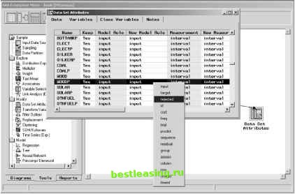Figure 17.5 SAS Enterprise Miner has a wide range of available model roles.

Variable Measures

Variables appear in data and have some important properties. Although databases are concerned with the type of variables (and well return to this topic in a moment), data mining is concerned with the measure of variables. It is the measure that determines how the algorithms treat the values. The following measures are important for data mining:

Categorical variables can be compared for equality but there is no meaningful ordering. For example, state abbreviations are categorical. The fact that Alabama is next to Alaska alphabetically does not mean that they are closer to each other than Alabama and Tennessee, which share a geographic border but appear much further apart alphabetically.

Ordered variables can be compared with equality and with greater than and less than. Classroom grades, which range from A to F, are an example of ordered values.

Interval variables are ordered and support the operation of subtraction (although not necessarily any other mathematical operation such as addition and multiplication). Dates and temperatures are examples of intervals.

True numeric variables are interval variables that support addition and other mathematical operations. Monetary amounts and customer tenure (measured in days) are examples of numeric variables.

The difference between true numerics and intervals is subtle. However, data mining algorithms treat both of these the same way. Also, note that these measures form a hierarchy. Any ordered variable is also categorical, any interval is also categorical, and any numeric is also interval.

There is a difference between measure and data type. A numeric variable, for instance, might represent a coding scheme-say for account status or even for state abbreviations. Although the values look like numbers, they are really categorical. Zip codes are a common example of this phenomenon.

Some algorithms expect variables to be of a certain measure. Statistical regression and neural networks, for instance, expect their inputs to be numeric. So, if a zip code field is included and stored as a number, then the algorithms treat its values as numeric, generally not a good approach. Decision trees, on the other hand, treat all their inputs as categorical or ordered, even when they are numbers.

Measure is one important property. In practice, variables have associated types in databases and file layouts. The following sections talk about data types and measures in more detail.

Numbers

Numbers usually represent quantities and are good variables for modeling purposes. Numeric quantities have both an ordering (which is used by decision trees) and an ability to perform arithmetic (used by other algorithms such as clustering and neural networks). Sometimes, what looks like a number really represents a code or an ID. In such cases, it is better to treat the number as a categorical value (discussed in the next two sections), since the ordering and arithmetic properties of the numbers may mislead data mining algorithms attempting to find patterns.

There are many different ways to transform numeric quantities. Figure 17.6 illustrates several common methods:

Normalization. The resulting values are made to fall within a certain range, for example, by subtracting the minimum value and dividing by the range. This process does not change the form of the distribution of the values. Normalization can be useful when using techniques that perform mathematical operations such as multiplication directly on the values, such as neural networks and K-means clustering. Decision trees are unaffected by normalization, since the normalization does not change the order of the values.

7,000 6,000 5,000 4,000 3,000 2,000 1,000 0

Original Data

Time

1.0 0.8 0.6 0.4 0.2 0.0

Normalized to [0, 1]

Time

Standardized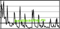

Time

Binned as Deciles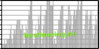

Time

Figure 17.6 Normalization, standardization, and binning are typical ways to transform a numeric variable.

Standardization. This transforms the values into the number of standard deviations from the mean, which gives a good sense of how unexpected the value is. The arithmetic is easy-subtract the average value and divide by the standard deviation. These standardized values are also called z-scores. As with normalization, standardization does not affect the ordering, so it has no effect on decision trees.

Equal-width binning. This transforms the variables into ranges that are fixed in width. The resulting variable has roughly the same distribution as the original variable. However, binning values affects all data mining algorithms.

Equal-height binning. This transforms the variables into n-tiles (such as quintiles or deciles) so that the same number of records falls into each bin. The resulting variable has a uniform distribution.

Perhaps unexpectedly, binning values can improve the performance of data mining algorithms. In the case of neural networks, binning is one of several ways of reducing the influence of outliers, because all outliers are grouped together into the same bin. In the case of decision trees, binned variables may result in child nodes having more equal sizes at high levels of the tree (that is, instead of one child getting 5 percent of the records and the other 95 percent, with the corresponding binned variable one might get 20 percent and the other 80 percent). Although the split on the binned variables is not optimal, subsequent splits may produce better trees.

о Ф □