

|
|

|
Промышленный лизинг
Методички
When the lookup table is small enough, such as Table 17.3, which describes the mapping between initial digits of a credit card number and the credit card type, then a simple formula can suffice for the lookup. The more common situation is having a secondary table or file with the information. This table might, for instance, contain: Populations and median household incomes of zip codes (usefully provided for downloading for the United States by the U.S. Census Bureau at www.census.gov) Hierarchies for product codes Store type information about retail locations Unfortunately data mining tools do not, as a rule, make it easy to do lookups without programming. Tools that do provide this facility, such as I-Miner from Insightful, usually require that both tables be sorted by the field or fields used for the lookup; an example of this is shown in Figure 17.12. This is palatable for one such field, but it is cumbersome when there are many different fields to be looked up. In general, it is easier to do these lookups outside the tool, especially when the lookup tables and original data are both coming from databases. Figure 17.12 Insightful Miner enables users to use and create lookup tables from the graphical user interface. 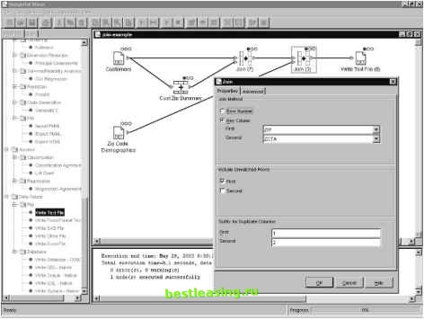 Sometimes, the lookup tables already exist. Other times, they must be created as needed. For instance, one useful predictor of customer attrition is the historical attrition rate by zip code. To add this to a customer signature requires calculating the historical attrition rate for each zip code and then using the result as a lookup table. WARNING When using database joins to look up values in a lookup table, always use a left outer join to ensure that no customer rows are lost in the process! An outer join in SQL looks like: SELECT c.*. Lvalue FROM (customer c left outer join lookup l on c.code = l.code) Table 17.3 Credit Card Prefixes
Pivoting Regular Time Series Data about customers is often stored at a monthly level, where each month has a separate row of data. For instance, billing data is often stored this way, since most subscription-based companies bill customers once a month. This data is an example of a regular time series, because the data occurs at fixed, defined intervals. Figure 17.13 illustrates the process needed to put this data into a customer signature. The data must be pivoted, so values that start out in rows end up in columns. This is generally a cumbersome process, because neither data mining tools nor SQL makes it easy to do pivoting. Data mining tools generally require programming for pivoting. To accomplish this, the customer file needs to be sorted by customer ID, and the billing file needs to be sorted by the customer ID and the billing date. Then, special-purpose code is needed to calculate the pivoting columns. In SAS, proc TRANSPOSE is used for this purpose. The sidebar Pivoting Data in SQL shows how it is done in SQL. Most businesses store customer data on a monthly basis, usually by calendar month. Some industries, though, show strong weekly cyclical patterns, because customers either do or do not do things over the weekend. For instance, Web sites might be most active during weekdays, and newspaper subscriptions generally start on Mondays or Sundays. Such weekly cycles interfere with the monthly data, because some months are longer than others. Consider a Web site where most activity is on weekdays. Some months have 20 weekdays; others have up to 23 (not including holidays). The difference between successive months could be 15 percent, due solely to the difference in the number of weekdays. To take this into account, divide the monthly activity by the number of weekdays during the month, to get an activity per weekday. This only makes sense, though, when there are strong weekly cycles.

Figure 17.13 Pivoting a field takes values stored in one or more rows for each customer and puts them into a single row for each customer, but in different columns. Team-Ffy® 1 2 3 4 5 6 7 8 9 10 11 12 13 14 15 16 17 18 19 20 21 22 23 24 25 26 27 28 29 30 31 32 33 34 35 36 37 38 39 40 41 42 43 44 45 46 47 48 49 50 51 52 53 54 55 56 57 58 59 60 61 62 63 64 65 66 67 68 69 70 71 72 73 74 75 76 77 78 79 80 81 82 83 84 85 86 87 88 89 90 91 92 93 94 95 96 97 98 99 100 101 102 103 104 105 106 107 108 109 110 111 112 113 114 115 116 117 118 119 120 121 122 123 124 125 126 127 128 129 130 131 132 133 134 135 136 137 138 139 140 141 142 143 144 145 146 147 148 149 150 151 152 153 154 155 156 157 158 159 160 161 162 163 164 165 166 167 168 169 170 171 172 173 174 175 176 177 178 179 180 181 182 183 184 185 186 187 188 189 190 191 192 193 194 195 196 197 [ 198 ] 199 200 201 202 203 204 205 206 207 208 209 210 211 212 213 214 215 216 217 218 219 220 221 222 |
|||||||||||||||||||||||||||||||||||||||||||||||||||||||||||||||||||||||||||||||||||||||||||||||||||||||||