One method of calculating frequency would be to take the length of time indicated by the historical data and divide it by the number of times the customer made a purchase. So, if the catalog data goes back 6 years and a customer made a single purchase, then that frequency would be once every 6 years.

Although simple, this approach misses an important point. Consider two customers:

John made a purchase 6 years ago and has received every catalog since then.

Mary made a purchase last month when she first received the catalog.

Does it make sense that both these customers have the same frequency? No. John more clearly has a frequency of no more than once every 6 years. Mary only had the opportunity to make one purchase in the past month, so her frequency would more accurately be described as once per month. The first point about frequency is that it should be measured from the first point in time that a customer had an opportunity to make a purchase.

There is another problem. What we really know about John and Mary is that their frequencies are no more than once every 6 years and no more than once per month, respectively. Historically, one observation does not contain enough information to deduce a real frequency. This is really a time to event problem, such as those discussed in Chapter 12.

Our goal here is to characterize frequency as a derived variable, rather than predict the next event (which is best approached using survival analysis). To do this, lets assume that there are two or more events, so the average time between events is the total span of time divided by the number of events minus one, as shown in Figure 17.14. This provides the average time between events for the period when the events occurred.

There is no perfect solution to the question of frequency, because customer events occur irregularly and we do not know what will happen in the future- the data is censored. Taking the time span from the first event to the most recent event runs into the problem that customers whose events all took place long ago may have a high frequency. The alternative is to take the time since the first event, in essence pretending that the present is an event. This is unsatisfying, because the next event is not known, and care must be taken when working with censored data. In practice, taking the number of events since the first event could have happened and dividing by the total span of time (or the span when the customer was active) is the best solution.

Purchase

First Contact

Frequency is 2 / (C -A), but does not include time after C

Frequeicy is 3 / C, but does not include time after C

Frequency is 3 / (D - A), but data is censored

Current Time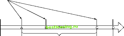

Frequency is 3/D, but data is censored Figure 17.14 There is no perfect way to estimate frequency, but these four ways are all reasonable.

Declining Usage

In telecommunications, one significant predictor of churn is declining usage- customers who use services less and less over time are more likely to leave than other customers. Customers who have declining usage are likely to have many variables indicating this:

Billing measures, such as recent amounts spent are quite small.

Usage measures, such as recent amounts used are quite small or always at monthly minimums.

Optional services recently have no usage.

Ratios of recent measures to older measures are less than 1, often significantly less than one, indicating recent usage is smaller than historical usage.

The existence of so many different measures for the same underlying behavior suggests a situation where a derived variable might be useful to capture the behavior in a single variable. The goal is to incorporate as much information as possible into a declining usage indicator.

When many different variables all suggest a single customer behavior, then it is likely that a derived variable that incorporates this information will do a better job for data mining.

Fortunately, mathematics provides an elegant solution, in the form of the best fit line, as shown in Figure 17.15. The goodness of fit is described by the R2 statistic, which varies from 0 to 1, with values near 0 being poor fit and values near 1 being very good. The slope of the line provides the average rate of increase or decrease in some variable over time. In statistics, this slope is called the beta function and is calculated according to the following formula:

Sum of (x-average(x))*(y-average(y)) / sum((x-average(x))2)

To give an example of how this might be used, consider the following data for the customer shown in the previous figure. Table 17.4 walks through the calculation for a typical customer.

Table 17.4 Example of Calculating the Slope for a Time Series