like. Data preparation is such an important topic that our colleague Dorian Pyle has written a book about it, Data Preparation for Data Mining (Morgan Kaufmann 1999), which should be on the bookshelf of every data miner. In this book, these issues are addressed in Chapter 17. Here are a few examples of such transformations.

Capture Trends

Most corporate data contains time series. Monthly snapshots of billing information, usage, contacts, and so on. Most data mining algorithms do not understand time series data. Signals such as three months of declining revenue cannot be spotted treating each months observation independently. It is up to the data miner to bring trend information to the surface by adding derived variables such as the ratio of spending in the most recent month to spending the month before for a short-term trend and the ratio of the most recent month to the same month a year ago for a long-term trend.

Create Ratios and Other Combinations of Variables

Trends are one example of bringing information to the surface by combining multiple variables. There are many others. Often, these additional fields are derived from the existing ones in ways that might be obvious to a knowledgeable analyst, but are unlikely to be considered by mere software. Typical examples include:

obesity index = height2 / weight PE = price / earnings pop density = population / area rpm = revenue passengers * miles

Adding fields that represent relationships considered important by experts in the field is a way of letting the mining process benefit from that expertise.

Convert Counts to Proportions

Many datasets contain counts or dollar values that are not particularly interesting in themselves because they vary according to some other value. Larger households spend more money on groceries than smaller households. They spend more money on produce, more money on meat, more money on packaged goods, more money on cleaning products, more money on everything. So comparing the dollar amount spent by different households in any one

category, such as bakery, will only reveal that large households spend more. It is much more interesting to compare the proportion of each households spending that goes to each category.

The value of converting counts to proportions can be seen by comparing two charts based on the NY State towns dataset. Figure 3.9 compares the count of houses with bad plumbing to the prevalence of heating with wood. A relationship is visible, but it is not strong. In Figure 3.10, where the count of houses with bad plumbing has been converted into the proportion of houses with bad plumbing, the relationship is much stronger. Towns where many houses have bad plumbing also have many houses heated by wood. Does this mean that wood smoke destroys plumbing? It is important to remember that the patterns that we find determine correlation, not causation.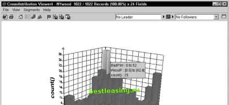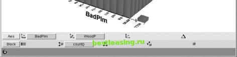

Figure 3.9 Chart comparing count of houses with bad plumbing to prevalence of heating with wood.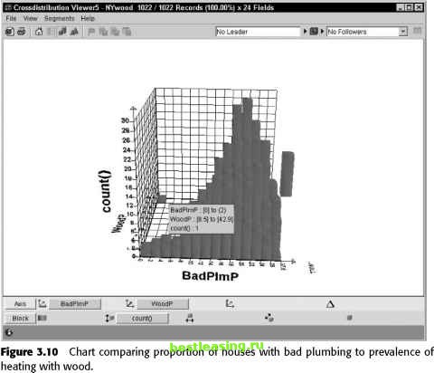

Step Seven: Build Models

The details of this step vary from technique to technique and are described in the chapters devoted to each data mining method. In general terms, this is the step where most of the work of creating a model occurs. In directed data mining, the training set is used to generate an explanation of the independent or target variable in terms of the independent or input variables. This explanation may take the form of a neural network, a decision tree, a linkage graph, or some other representation of the relationship between the target and the other fields in the database. In undirected data mining, there is no target variable. The model finds relationships between records and expresses them as association rules or by assigning them to common clusters.

Building models is the one step of the data mining process that has been truly automated by modern data mining software. For that reason, it takes up relatively little of the time in a data mining project.