The standard way of describing the accuracy of an estimation model is by measuring how far off the estimates are on average. But, simply subtracting the estimated value from the true value at each point and taking the mean results in a meaningless number. To see why, consider the estimates in Table 3.1.

The average difference between the true values and the estimates is zero; positive differences and negative differences have canceled each other out. The usual way of solving this problem is to sum the squares of the differences rather than the differences themselves. The average of the squared differences is called the variance. The estimates in this table have a variance of 10.

(-52 + 22 + -22 + 12 + 42 )/5 = (25 + 4 + 4 + 1 + 16)/5 = 50/5 = 10

The smaller the variance, the more accurate the estimate. A drawback to variance as a measure is that it is not expressed in the same units as the estimates themselves. For estimated prices in dollars, it is more useful to know how far off the estimates are in dollars rather than square dollars! For that reason, it is usual to take the square root of the variance to get a measure called the standard deviation. The standard deviation of these estimates is the square root of 10 or about 3.16. For our purposes, all you need to know about the standard deviation is that it is a measure of how widely the estimated values vary from the true values.

Comparing Models Using Lift

Directed models, whether created using neural networks, decision trees, genetic algorithms, or Ouija boards, are all created to accomplish some task. Why not judge them on their ability to classify, estimate, and predict? The most common way to compare the performance of classification models is to use a ratio called lift. This measure can be adapted to compare models designed for other tasks as well. What lift actually measures is the change in concentration of a particular class when the model is used to select a group from the general population.

lift = P(classt sample) / P(classt population)

Table 3.1 Countervailing Errors

An example helps to explain this. Suppose that we are building a model to predict who is likely to respond to a direct mail solicitation. As usual, we build the model using a preclassified training dataset and, if necessary, a preclassi-fied validation set as well. Now we are ready to use the test set to calculate the models lift.

The classifier scores the records in the test set as either predicted to respond or not predicted to respond. Of course, it is not correct every time, but if the model is any good at all, the group of records marked predicted to respond contains a higher proportion of actual responders than the test set as a whole. Consider these records. If the test set contains 5 percent actual responders and the sample contains 50 percent actual responders, the model provides a lift of 10 (50 divided by 5).

Is the model that produces the highest lift necessarily the best model? Surely a list of people half of whom will respond is preferable to a list where only a quarter will respond, right? Not necessarily-not if the first list has only 10 names on it! \К\\>

The point is that lift is a function of sample size. If the classifier only picks out 10 likely respondents, and it is right 100 percent of the time, it will achieve a lift of 20-the highest lift possible when the population contains 5 percent responders. As the confidence level required to classify someone as likely to respond is relaxed, the mailing list gets longer, and the lift decreases.

Charts like the one in Figure 3.13 will become very familiar as you work with data mining tools. It is created by sorting all the prospects according to their likelihood of responding as predicted by the model. As the size of the mailing list increases, we reach farther and farther down the list. The X-axis shows the percentage of the population getting our mailing. The Y-axis shows the percentage of all responders we reach.

If no model were used, mailing to 10 percent of the population would reach 10 percent of the responders, mailing to 50 percent of the population would reach 50 percent of the responders, and mailing to everyone would reach all the responders. This mass-mailing approach is illustrated by the line slanting upwards. The other curve shows what happens if the model is used to select recipients for the mailing. The model finds 20 percent of the responders by mailing to only 10 percent of the population. Soliciting half the population reaches over 70 percent of the responders.

Charts like the one in Figure 3.13 are often referred to as lift charts, although what is really being graphed is cumulative response or concentration. Figure 3.13 shows the actual lift chart corresponding to the response chart in Figure 3.14. The chart shows clearly that lift decreases as the size of the target list increases.

Team-Fly®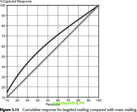

Problems with Lift

Lift solves the problem of how to compare the performance of models of different kinds, but it is still not powerful enough to answer the most important questions: Is the model worth the time, effort, and money it cost to build it? Will mailing to a segment where lift is 3 result in a profitable campaign?

These kinds of questions cannot be answered without more knowledge of the business context, in order to build costs and revenues into the calculation. Still, lift is a very handy tool for comparing the performance of two models applied to the same or comparable data. Note that the performance of two models can only be compared using lift when the tests sets have the same density of the outcome.