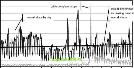May Jun Jul Aug Sep Oct Nov Dec Jan Feb Mar Apr May Jun

Figure 5.2 This chart shows two time series plotted with different scales. The dark line is for overall stops; the light line for pricing related stops shows the impact of a change in pricing strategy at the end of January.

Standardized Values

A time series chart provides useful information. However, it does not give an idea as to whether the changes over time are expected or unexpected. For this, we need some tools from statistics.

One way of looking at a time series is as a partition of all the data, with a little bit on each day. The statistician now wants to ask a skeptical question: Is it possible that the differences seen on each day are strictly due to chance? This is the null hypothesis, which is answered by calculating the p-value-the probability that the variation among values could be explained by chance alone.

Statisticians have been studying this fundamental question for over a century. Fortunately, they have also devised some techniques for answering it. This is a question about sample variation. Each day represents a sample of stops from all the stops that occurred during the period. The variation in stops observed on different days might simply be due to an expected variation in taking random samples.

There is a basic theorem in statistics, called the Central Limit Theorem, which says the following:

As more and more samples are taken from a population, the distribution of the averages of the samples (or a similar statistic) follows the normal distribution. The average (what statisticians call the mean) of the samples comes arbitrarily close to the average of the entire population.

The Central Limit Theorem is actually a very deep theorem and quite interesting. More importantly, it is useful. In the case of discrete variables, such as number of customers who stop on each day, the same idea holds. The statistic used for this example is the count of the number of stops on each day, as shown earlier in Figure 5.2. (Strictly speaking, it would be better to use a proportion, such as the ratio of stops to the number of customers; this is equivalent to the count for our purposes with the assumption that the number of customers is constant over the period.)

The normal distribution is described by two parameters, the mean and the standard deviation. The mean is the average count for each day. The standard deviation is a measure of the extent to which values tend to cluster around the mean and is explained more fully later in the chapter; for now, using a function such as STDEV() in Excel or STDDEV() in SQL is sufficient. For the time series, the standard deviation is the standard deviation of the daily counts. Assuming that the values for each day were taken randomly from the stops for the entire period, the set of counts should follow a normal distribution. If they dont follow a normal distribution, then something besides chance is affecting the values. Notice that this does not tell us what is affecting the values, only that the simplest explanation, sample variation, is insufficient to explain them.

This is the motivation for standardizing time series values. This process produces the number of standard deviations from the average:

Calculate the average value for all days.

Calculate the standard deviation for all days.

For each value, subtract the average and divide by the standard deviation to get the number of standard deviations from the average.

The purpose of standardizing the values is to test the null hypothesis. When true, the standardized values should follow the normal distribution (with an average of 0 and a standard deviation of 1), exhibiting several useful properties. First, the standardized value should take on negative values and positive values with about equal frequency. Also, when standardized, about two-thirds (68.4 percent) of the values should be between minus one and one. A bit over 95 percent of the values should be between -2 and 2. And values over 3 or less than -3 should be very, very rare-probably not visible in the data. Of course, should here means that the values are following the normal distribution and the null hypothesis holds (that is, all time related effects are explained by sample variation). When the null hypothesis does not hold, it is often apparent from the standardized values. The aside, A Question of Terminology, talks a bit more about distributions, normal and otherwise.

Figure 5.3 shows the standardized values for the data in Figure 5.2. The first thing to notice is that the shape of the standardized curve is very similar to the shape of the original data; what has changed is the scale on the vertical dimension. When comparing two curves, the scales for each change. In the previous

figure, overall stops were much larger than pricing stops, so the two were shown using different scales. In this case, the standardized pricing stops are towering over the standardized overall stops, even though both are on the same scale.

The overall stops in Figure 5.3 are pretty typically normal, with the following caveats. There is a large peak in December, which probably needs to be explained because the value is over four standard deviations away from the average. Also, there is a strong weekly trend. It would be a good idea to repeat this chart using weekly stops instead of daily stops, to see the variation on the weekly level.

The lighter line showing the pricing related stops clearly does not follow the normal distribution. Many more values are negative than positive. The peak is at over 13-which is way, way too high.

Standardized values, or z-values as they are often called, are quite useful. This example has used them for looking at values over time too see whether the values look like they were taken randomly on each day; that is, whether the variation in daily values could be explained by sampling variation. On days when the z-value is relatively high or low, then we are suspicious that something else is at work, that there is some other factor affecting the stops. For instance, the peak in pricing stops occurred because there was a change in pricing. The effect is quite evident in the daily z-values.

The z-value is useful for other reasons as well. For instance, it is one way of taking several variables and converting them to similar ranges. This can be useful for several data mining techniques, such as clustering and neural networks. Other uses of the z-value are covered in Chapter 17, which discusses data transformations.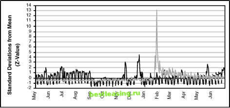

Figure 5.3 Standardized values make it possible to compare different groups on the same chart using the same scale; this shows overall stops and price increase related stops.