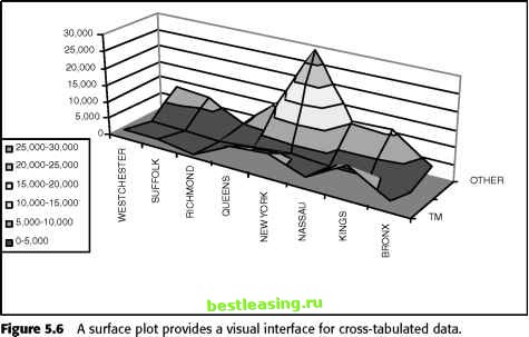
-5 -4 -3 -2 -1 0 1 2 3 4 5

Z-Value

Figure 5.4 The tail of the normal distribution answers the question: What is the probability of getting a value of z or greater?

Figure 5.5 shows the signed confidence for the data shown earlier in Figures 5.2 and 5.3, using the two-tailed probability. The shape of the signed confidence is different from the earlier shapes. The overall stops bounce around, usually remaining within reasonable bounds. The pricing-related stops, though, once again show a very distinct pattern, being too low for a long time, then peaking and descending. The signed confidence levels are bounded by 100 percent and -100 percent. In this chart, the extreme values are near 100 percent or -100 percent, and it is hard to tell the difference between 99.9 percent and 99.99999 percent. To distinguish values near the extremes, the z-values in Figure 5.3 are better than the signed confidence.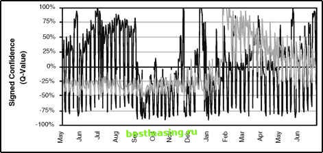

Figure 5.5 Based on the same data from Figures 5.2 and 5.3, this chart shows the signed confidence (q-values) of the observed value based on the average and standard deviation. This sign is positive when the observed value is too high, negative when it is too low.

Cross-Tabulations

Time series are an example of cross-tabulation-looking at the values of two or more variables at one time. For time series, the second variable is the time something occurred.

Table 5.1 shows an example used later in this chapter. The cross-tabulation shows the number of new customers from counties in southeastern New York state by three channels: telemarketing, direct mail, and other. This table shows both the raw counts and the relative frequencies.

It is possible to visualize cross-tabulations as well. However, there is a lot of data being presented, and some people do not follow complicated pictures. Figure 5.6 shows a surface plot for the counts shown in the table. A surface plot often looks a bit like hilly terrain. The counts are the height of the hills; the counties go up one side and the channels make the third dimension. This surface plot shows that the other channel is quite high for Manhattan (New York county). Although not a problem in this case, such peaks can hide other hills and valleys on the surface plot.

Looking at Continuous Variables

Statistics originated to understand the data collected by scientists, most of which took the form of continuous measurements. In data mining, we encounter continuous data less often, because there is a wealth of descriptive data as well. This section talks about continuous data from the perspective of descriptive statistics.

Table 5.1 Cross-tabulation of Starts by County and Channel

Statistical Measures for Continuous Variables

The most basic statistical measures describe a set of data with just a single value. The most commonly used statistic is the mean or average value (the sum of all the values divided by the number of them). Some other important things

to look at are:

Range. The range is the difference between the smallest and largest observation in the sample. The range is often looked at along with the minimum and maximum values themselves.

Mean. This is what is called an average in everyday speech.

Median. The median value is the one which splits the observations into two equally sized groups, one having observations smaller than the median and another containing observations larger than the median.

Mode. This is the value that occurs most often.

The median can be used in some situations where it is impossible to calculate the mean, such as when incomes are reported in ranges of $10,000 dollars with a final category over $100,000. The number of observations are known in each group, but not the actual values. In addition, the median is less affected by a few observations that are out of line with the others. For instance, if Bill Gates moves onto your block, the average net worth of the neighborhood will dramatically increase. However, the median net worth may not change at all.