In addition, various ways of characterizing the range are useful. The range itself is defined by the minimum and maximum value. It is often worth looking at percentile information, such as the 25th and 75th percentile, to understand the limits of the middle half of the values as well.

Figure 5.7 shows a chart where the range and average are displayed for order amount by day. This chart uses a logarithmic (log) scale for the vertical axis, because the minimum order is under $10 and the maximum over $1,000. In fact, the minimum is consistently around $10, the average around $70, and the maximum around $1,000. As with discrete variables, it is valuable to use a time chart for continuous values to see when unexpected things are happening.

Variance and Standard Deviation

Variance is a measure of the dispersion of a sample or how closely the observations cluster around the average. The range is not a good measure of dispersion because it takes only two values into account-the extremes. Removing one extreme can, sometimes, dramatically change the range. The variance, on the other hand, takes every value into account. The difference between a given observation and the mean of the sample is called its deviation. The variance is defined as the average of the squares of the deviations.

Standard deviation, the square root of the variance, is the most frequently used measure of dispersion. It is more convenient than variance because it is expressed in the same units as the observations rather than in terms of those units squared. This allows the standard deviation itself to be used as a unit of measurement. The z-score, which we used earlier, is an observations distance from the mean measured in standard deviations. Using the normal distribution, the z-score can be converted to a probability or confidence level.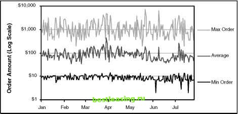

Figure 5.7 A time chart can also be used for continuous values; this one shows the range and average for order amounts each day.

A Couple More Statistical Ideas

Correlation is a measure of the extent to which a change in one variable is related to a change in another. Correlation ranges from -1 to 1. A correlation of 0 means that the two variables are not related. A correlation of 1 means that as the first variable changes, the second is guaranteed to change in the same direction, though not necessarily by the same amount. Another measure of correlation is the R2 value, which is the correlation squared and goes from 0 (no relationship) to 1 (complete relationship). For instance, the radius and the circumference of a circle are perfectly correlated, although the latter grows faster than the former. A negative correlation means that the two variables move in opposite directions. For example, altitude is negatively correlated to air pressure.

Regression is the process of using the value of one of a pair of correlated variables in order to predict the value of the second. The most common form of regression is linear regression, so called because it attempts to fit a straight line through the observed X and Y pairs in a sample. Once the line has been established, it can be used to predict a value for Y given any X and for X given any Y.

Measuring Response

This section looks at statistical ideas in the context of a marketing campaign. The champion-challenger approach to marketing tries out different ideas against the business as usual. For instance, assume that a company sends out a million billing inserts each month to entice customers to do something. They have settled on one approach to the bill inserts, which is the champion offer. Another offer is a challenger to this offer. Their approach to comparing these is:

Send the champion offer to 900,000 customers.

Send the challenger offer to 100,000 customers.

Determine which is better.

The question is, how do we know when one offer is better than another? This section introduces the ideas of confidence to understand this in more detail.

Standard Error of a Proportion

The approach to answering this question uses the idea of a confidence interval. The challenger offer, in the above scenario, is being sent to a random subset of customers. Based on the response in this subset, what is the expected response for this offer for the entire population?

For instance, lets assume that 50,000 people in the original population would have responded to the challenger offer if they had received it. Then about 5,000 would be expected to respond in the 10 percent of the population that received

the challenger offer. If exactly this number did respond, then the sample response rate and the population response rate would both be 5.0 percent. However, it is possible (though highly, highly unlikely) that all 50,000 responders are in the sample that receives the challenger offer; this would yield a response rate of 50 percent. On the other hand it is also possible (and also highly, highly unlikely) that none of the 50,000 are in the sample chosen, for a response rate of 0 percent. In any sample of one-tenth the population, the observed response rate might be as low as 0 percent or as high as 50 percent. These are the extreme values, of course; the actual value is much more likely to be close to 5 percent.

So far, the example has shown that there are many different samples that can be pulled from the population. Now, lets flip the situation and say that we have observed 5,000 responders in the sample. What does this tell us about the entire population? Once again, it is possible that these are all the responders in the population, so the low-end estimate is 0.5 percent. On the other hand, it is possible that everyone else was as responder and we were very, very unlucky in choosing the sample. The high end would then be 90.5 percent.

That is, there is a 100 percent confidence that the actual response rate on the population is between 0.5 percent and 90.5 percent. Having a high confidence is good; however, the range is too broad to be useful. We are willing to settle for a lower confidence level. Often, 95 or 99 percent confidence is quite sufficient for marketing purposes.

The distribution for the response values follows something called the binomial distribution. Happily, the binomial distribution is very similar to the normal distribution whenever we are working with a population larger than a few hundred people. In Figure 5.8, the jagged line is the binomial distribution and the smooth line is the corresponding normal distribution; they are practically identical.

The challenge is to determine the corresponding normal distribution given that a sample of size 100,000 had a response rate of 5 percent. As mentioned earlier, the normal distribution has two parameters, the mean and standard deviation. The mean is the observed average (5 percent) in the sample. To calculate the standard deviation, we need a formula, and statisticians have figured out the relationship between the standard deviation (strictly speaking, this is the standard error but the two are equivalent for our purposes) and the mean value and the sample size for a proportion. This is called the standard error of a proportion (SEP) and has the formula:

In this formula, p is the average value and N is the size of the population. So, the corresponding normal distribution has a standard deviation equal to the square root of the product of the observed response times one minus the observed response divided by the total number of samples.

We have already observed that about 68 percent of data following a normal distribution lies within one standard deviation. For the sample size of 100,000, the

SEP =