

|
|

|
Промышленный лизинг
Методички
The appeal of the chi-square test is that it readily adapts to multiple test groups and multiple outcomes, so long as the different groups are distinct from each other. This, in fact, is about the only important rule when using this test. As described in the next chapter on decision trees, the chi-square test is the basis for one of the earliest forms of decision trees. Expected Values The place to start with chi-square is to lay data out in a table, as in Table 5.5. This is a simple 2 x 2 table, which represents a test group and a control group in a test that has two outcomes, say response and nonresponse. This table also shows the total values for each column and row; that is, the total number of responders and nonresponders (each column) and the total number in the test and control groups (each row). The response column is added for reference; it is not part of the calculation. What if the data were broken up between these groups in a completely unbiased way? That is, what if there really were no differences between the columns and rows in the table? This is a completely reasonable question. We can calculate the expected values, assuming that the number of responders and non-responders is the same, and assuming that the sizes of the champion and challenger groups are the same. That is, we can calculate the expected value in each cell, given that the size of the rows and columns are the same as in the original data. One way of calculating the expected values is to calculate the proportion of each row that is in each column, by computing each of the following four quantities, as shown in Table 5.6: Proportion of everyone who responds Proportion of everyone who does not respond These proportions are then multiplied by the count for each row to obtain the expected value. This method for calculating the expected value works when the tabular data has more columns or more rows. Table 5.5 The Champion-Challenger Data Laid out for the Chi-Square Test
Table 5.6 Calculating the Expected Values and Deviations from Expected for the Data in Table 5.5
The expected value is quite interesting, because it shows how the data would break up if there were no other effects. Notice that the expected value is measured in the same units as each cell, typically a customer count, so it actually has a meaning. Also, the sum of the expected values is the same as the sum of all the cells in the original table. The table also includes the deviation, which is the difference between the observed value and the expected value. In this case, the deviations all have the same value, but with different signs. This is because the original data has two rows and two columns. Later in the chapter there are examples using larger tables where the deviations are different. However, the deviations in each row and each column always cancel out, so the sum of the deviations in each row is always 0. Chi-Square Value The deviation is a good tool for looking at values. However, it does not provide information as to whether the deviation is expected or not expected. Doing this requires some more tools from statistics, namely, the chi-square distribution developed by the English statistician Karl Pearson in 1900. The chi-square value for each cell is simply the calculation: . , . (x - expected(x)) exp ected(x) The chi-square value for the entire table is the sum of the chi-square values of all the cells in the table. Notice that the chi-square value is always 0 or positive. Also, when the values in the table match the expected value, then the overall chi-square is 0. This is the best that we can do. As the deviations from the expected value get larger in magnitude, the chi-square value also gets larger. Unfortunately, chi-square values do not follow a normal distribution. This is actually obvious, because the chi-square value is always positive, and the normal distribution is symmetric. The good news is that chi-square values follow another distribution, which is also well understood. However, the chi-square distribution depends not only on the value itself but also on the size of the table. Figure 5.9 shows the density functions for several chi-square distributions. What the chi-square depends on is the degrees of freedom. Unlike many ideas in probability and statistics, degrees of freedom is easier to calculate than to explain. The number of degrees of freedom of a table is calculated by subtracting one from the number of rows and the number of columns and multiplying them together. The 2 x 2 table in the previous example has 1 degree of freedom. A 5 x 7 table would have 24 (4 * 6) degrees of freedom. The aside Degrees of Freedom discusses this in a bit more detail. WARNINGThe chi-square test does not work when the number of expected values in any cell is less than 5 (and we prefer a slightly higher bound). Although this is not an issue for large data mining problems, it can be an issue when analyzing results from a small test. The process for using the chi-square test is: Calculate the expected values. Calculate the deviations from expected. Calculate the chi-square (square the deviations and divide by the expected). Sum for an overall chi-square value for the table. Calculate the probability that the observed values are due to chance (in Excel, you can use the CHIDIST function). 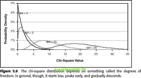 Team-Fly® 1 2 3 4 5 6 7 8 9 10 11 12 13 14 15 16 17 18 19 20 21 22 23 24 25 26 27 28 29 30 31 32 33 34 35 36 37 38 39 40 41 42 43 44 45 46 47 48 49 50 51 52 53 54 55 56 57 [ 58 ] 59 60 61 62 63 64 65 66 67 68 69 70 71 72 73 74 75 76 77 78 79 80 81 82 83 84 85 86 87 88 89 90 91 92 93 94 95 96 97 98 99 100 101 102 103 104 105 106 107 108 109 110 111 112 113 114 115 116 117 118 119 120 121 122 123 124 125 126 127 128 129 130 131 132 133 134 135 136 137 138 139 140 141 142 143 144 145 146 147 148 149 150 151 152 153 154 155 156 157 158 159 160 161 162 163 164 165 166 167 168 169 170 171 172 173 174 175 176 177 178 179 180 181 182 183 184 185 186 187 188 189 190 191 192 193 194 195 196 197 198 199 200 201 202 203 204 205 206 207 208 209 210 211 212 213 214 215 216 217 218 219 220 221 222 |
||||||||||||||||||||||||||||||||||||||||||||||||||||||||||||