

|
|

|
Промышленный лизинг
Методички
Table 5.8 Chi-Square Calculation for Counties and Channels Example
Table 5.9 Chi-Square Calculation for Bronx and TM
The result is a set of chi-square values for the Bronx-TM combination, in a table with 1 degree of freedom. The Bronx-TM score by itself is a good approximation of the overall chi-square value for the 2 x 2 table (this assumes that the original cells are roughly the same size). The calculation for the chi-square value uses this value (1002.3) with 1 degree of freedom. Conveniently, the chi-square calculation for this cell is the same as the chi-square for the cell in the original calculation, although the other values do not match anything. This makes it unnecessary to do additional calculations. This means that an estimate of the effect of each combination of variables can be obtained using the chi-square value in the cell with a degree of freedom of 1. The result is a table that has a set of p-values that a given square is caused by chance, as shown in Table 5.10. However, there is a second correction that needs to be made because there are many comparisons taking place at the same time. Bonferronis adjustment takes care of this by multiplying each p-value by the number of comparisons- which is the number of cells in the table. For final presentation purposes, convert the p-values to their opposite, the confidence and multiply by the sign of the deviation to get a signed confidence. Figure 5.10 illustrates the result. Table 5.10 Estimated P-Value for Each Combination of County and Channel, without Correcting for Number of Comparisons
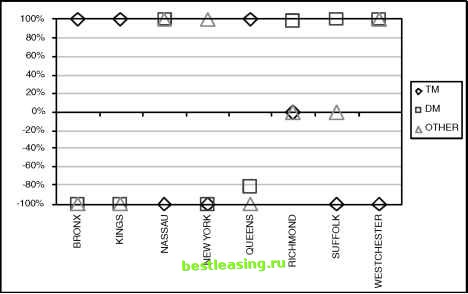 Figure 5.10 This chart shows the signed confidence values for each county and region combination; the preponderance of values near 100% and -100% indicate that observed differences are statistically significant. The result is interesting. First, almost all the values are near 100 percent or -100 percent, meaning that there are statistically significant differences among the counties. In fact, telemarketing (the diamond) and direct mail (the square) are always at opposite ends. There is a direct inverse relationship between the two. Direct mail is high and telemarketing low in three counties-Manhattan, Nassau, and Suffolk. There are many wealthy areas in these counties, suggesting that wealthy customers are more likely to respond to direct mail than telemarketing. Of course, this could also mean that direct mail campaigns are directed to these areas, and telemarketing to other areas, so the geography was determined by the business operations. To determine which of these possibilities is correct, we would need to know who was contacted as well as who responded. Data Mining and Statistics Many of the data mining techniques discussed in the next eight chapters were invented by statisticians or have now been integrated into statistical software; they are extensions of standard statistics. Although data miners and 1 2 3 4 5 6 7 8 9 10 11 12 13 14 15 16 17 18 19 20 21 22 23 24 25 26 27 28 29 30 31 32 33 34 35 36 37 38 39 40 41 42 43 44 45 46 47 48 49 50 51 52 53 54 55 56 57 58 59 [ 60 ] 61 62 63 64 65 66 67 68 69 70 71 72 73 74 75 76 77 78 79 80 81 82 83 84 85 86 87 88 89 90 91 92 93 94 95 96 97 98 99 100 101 102 103 104 105 106 107 108 109 110 111 112 113 114 115 116 117 118 119 120 121 122 123 124 125 126 127 128 129 130 131 132 133 134 135 136 137 138 139 140 141 142 143 144 145 146 147 148 149 150 151 152 153 154 155 156 157 158 159 160 161 162 163 164 165 166 167 168 169 170 171 172 173 174 175 176 177 178 179 180 181 182 183 184 185 186 187 188 189 190 191 192 193 194 195 196 197 198 199 200 201 202 203 204 205 206 207 208 209 210 211 212 213 214 215 216 217 218 219 220 221 222 |
||||||||||||||||||||||||||||||||||||||||||||||||||||||||||||||||||||||||||||||||||||||||||||||||||||||||||||||||||||||||||||||||||||||||||||||