

|
|

|
Промышленный лизинг
Методички
< 4.5 40% I num VOM orders i i < 1 > 1 I average $ demand 47.6 J 47.6 L avg $/month 50% tot units demand I-1-1 < 2 2.10132,4. > 4.116 [4.5, 15.5] days since last 221.5 I GMM buyer flag 0 1 I . I tot $ 9604 9.15, 4 I > 41.255 > 15.5 days since last 1 > 725 < 756 > 756 Figure 6.3 This ternary decision tree is applied to the same the same classification problem as in Figure 6.1. > < TIP There is no relationship between the number of branches allowed at a node and the number of classes in the target variable. A binary tree (that is, one with two-way splits) can be used to classify records into any number of categories, and a tree with multiway splits can be used to classify a binary target variable. How a Decision Tree Is Grown Although there are many variations on the core decision tree algorithm, all of them share the same basic procedure: Repeatedly split the data into smaller and smaller groups in such a way that each new generation of nodes has greater purity than its ancestors with respect to the target variable. For most of this discussion, we assume a binary, categorical target variable, such as responder/nonresponder. This simplifies the explanations without much loss of generality. Finding the Splits At the start of the process, there is a training set consisting of preclassified records-that is, the value of the target variable is known for all cases. The goal is to build a tree that assigns a class (or a likelihood of membership in each class) to the target field of a new record based on the values of the input variables. The tree is built by splitting the records at each node according to a function of a single input field. The first task, therefore, is to decide which of the input fields makes the best split. The best split is defined as one that does the best job of separating the records into groups where a single class predominates in each group. The measure used to evaluate a potential split is purity. The next section talks about specific methods for calculating purity in more detail. However, they are all trying to achieve the same effect. With all of them, low purity means that the set contains a representative distribution of classes (relative to the parent node), while high purity means that members of a single class predominate. The best split is the one that increases the purity of the record sets by the greatest amount. A good split also creates nodes of similar size, or at least does not create nodes containing very few records. These ideas are easy to see visually. Figure 6.4 illustrates some good and bad splits. Original Data
Poor Split Poor Split 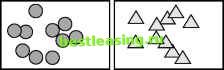 Good Split Figure 6.4 A good split increases purity for all the children. Team-Fly® The first split is a poor one because there is no increase in purity. The initial population contains equal numbers of the two sorts of dot; after the split, so does each child. The second split is also poor, because all though purity is increased slightly, the pure node has few members and the purity of the larger child is only marginally better than that of the parent. The final split is a good one because it leads to children of roughly same size and with much higher purity than the parent. Tree-building algorithms are exhaustive. They proceed by taking each input variable in turn and measuring the increase in purity that results from every split suggested by that variable. After trying all the input variables, the one that yields the best split is used for the initial split, creating two or more children. If no split is possible (because there are too few records) or if no split makes an improvement, then the algorithm is finished with that node and the node become a leaf node. Otherwise, the algorithm performs the split and repeats itself on each of the children. An algorithm that repeats itself in this way is called a recursive algorithm. Splits are evaluated based on their effect on node purity in terms of the target variable. This means that the choice of an appropriate splitting criterion depends on the type of the target variable, not on the type of the input variable. With a categorical target variable, a test such as Gini, information gain, or chi-square is appropriate whether the input variable providing the split is numeric or categorical. Similarly, with a continuous, numeric variable, a test such as variance reduction or the F-test is appropriate for evaluating the split regardless of whether the input variable providing the split is categorical or numeric. Splitting on a Numeric Input Variable When searching for a binary split on a numeric input variable, each value that the variable takes on in the training set is treated as a candidate value for the split. Splits on a numeric variable take the form X<N. All records where the value of X (the splitting variable) is less than some constant N are sent to one child and all records where the value of X is greater than or equal to N are sent to the other. After each trial split, the increase in purity, if any, due to the split is measured. In the interests of efficiency, some implementations of the splitting algorithm do not actually evaluate every value; they evaluate a sample of the values instead. When the decision tree is scored, the only use that it makes of numeric inputs is to compare their values with the split points. They are never multiplied by weights or added together as they are in many other types of models. This has the important consequence that decision trees are not sensitive to outliers or skewed distributions of numeric variables, because the tree only uses the rank of numeric variables and not their absolute values. 1 2 3 4 5 6 7 8 9 10 11 12 13 14 15 16 17 18 19 20 21 22 23 24 25 26 27 28 29 30 31 32 33 34 35 36 37 38 39 40 41 42 43 44 45 46 47 48 49 50 51 52 53 54 55 56 57 58 59 60 61 62 63 64 [ 65 ] 66 67 68 69 70 71 72 73 74 75 76 77 78 79 80 81 82 83 84 85 86 87 88 89 90 91 92 93 94 95 96 97 98 99 100 101 102 103 104 105 106 107 108 109 110 111 112 113 114 115 116 117 118 119 120 121 122 123 124 125 126 127 128 129 130 131 132 133 134 135 136 137 138 139 140 141 142 143 144 145 146 147 148 149 150 151 152 153 154 155 156 157 158 159 160 161 162 163 164 165 166 167 168 169 170 171 172 173 174 175 176 177 178 179 180 181 182 183 184 185 186 187 188 189 190 191 192 193 194 195 196 197 198 199 200 201 202 203 204 205 206 207 208 209 210 211 212 213 214 215 216 217 218 219 220 221 222 |