Purity and Diversity

The first edition of this book described splitting criteria in terms of the decrease in diversity resulting from the split. In this edition, we refer instead to the increase in purity, which seems slightly more intuitive. The two phrases refer to the same idea. A purity measure that ranges from 0 (when no two items in the sample are in the same class) to 1 (when all items in the sample are in the same class) can be turned into a diversity measure by subtracting it from 1. Some of the measures used to evaluate decision tree splits assign the lowest score to a pure node; others assign the highest score to a pure node. This discussion refers to all of them as purity measures, and the goal is to optimize purity by minimizing or maximizing the chosen measure.

Figure 6.5 shows a good split. The parent node contains equal numbers of light and dark dots. The left child contains nine light dots and one dark dot. The right child contains nine dark dots and one light dot. Clearly, the purity has increased, but how can the increase be quantified? And how can this split be compared to others? That requires a formal definition of purity, several of which are listed below.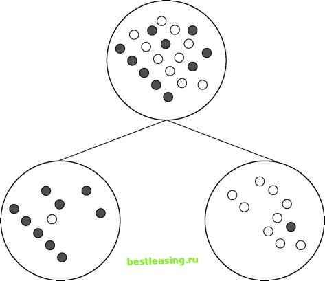

Figure 6.5 A good split on a binary categorical variable increases purity.

Purity measures for evaluating splits for categorical target variables include:

Gini (also called population diversity)

Entropy (also called information gain)

Information gain ratio

Chi-square test

When the target variable is numeric, one approach is to bin the value and use one of the above measures. There are, however, two measures in common use for numeric targets:

Reduction in variance

F test

Note that the choice of an appropriate purity measure depends on whether the target variable is categorical or numeric. The type of the input variable does not matter, so an entire tree is built with the same purity measure. The split illustrated in 6.5 might be provided by a numeric input variable (AGE > 46) or by a categorical variable (STATE is a member of CT, MA, ME, NH, RI, VT). The purity of the children is the same regardless of the type of split.

Gini or Population Diversity

One popular splitting criterion is named Gini, after Italian statistician and economist, Corrado Gini. This measure, which is also used by biologists and ecologists studying population diversity, gives the probability that two items chosen at random from the same population are in the same class. For a pure population, this probability is 1.

The Gini measure of a node is simply the sum of the squares of the proportions of the classes. For the split shown in Figure 6.5, the parent population has an equal number of light and dark dots. A node with equal numbers of each of 2 classes has a score of 0.52 + 0.52 = 0.5, which is expected because the chance of picking the same class twice by random selection with replacement is one out of two. The Gini score for either of the resulting nodes is 0.12 + 0.92 = 0.82. A perfectly pure node would have a Gini score of 1. A node that is evenly balanced would have a Gini score of 0.5. Sometimes the scores is doubled and then 1 subtracted, so it is between 0 and 1. However, such a manipulation makes no difference when comparing different scores to optimize purity.

To calculate the impact of a split, take the Gini score of each child node and multiply it by the proportion of records that reach that node and then sum the resulting numbers. In this case, since the records are split evenly between the two nodes resulting from the split and each node has the same Gini score, the score for the split is the same as for either of the two nodes.

Entropy Reduction or Information Gain

Information gain uses a clever idea for defining purity. If a leaf is entirely pure, then the classes in the leaf can be easily described-they all fall in the same class. On the other hand, if a leaf is highly impure, then describing it is much more complicated. Information theory, a part of computer science, has devised a measure for this situation called entropy. In information theory, entropy is a measure of how disorganized a system is. A comprehensive introduction to information theory is far beyond the scope of this book. For our purposes, the intuitive notion is that the number of bits required to describe a particular situation or outcome depends on the size of the set of possible outcomes. Entropy can be thought of as a measure of the number of yes/no questions it would take to determine the state of the system. If there are 16 possible states, it takes log2(16), or four bits, to enumerate them or identify a particular one. Additional information reduces the number of questions needed to determine the state of the system, so information gain means the same thing as entropy reduction. Both terms are used to describe decision tree algorithms.

The entropy of a particular decision tree node is the sum, over all the classes represented in the node, of the proportion of records belonging to a particular class multiplied by the base two logarithm of that proportion. (Actually, this sum is usually multiplied by -1 in order to obtain a positive number.) The entropy of a split is simply the sum of the entropies of all the nodes resulting from the split weighted by each nodes proportion of the records. When entropy reduction is chosen as a splitting criterion, the algorithm searches for the split that reduces entropy (or, equivalently, increases information) by the greatest amount.

For a binary target variable such as the one shown in Figure 6.5, the formula for the entropy of a single node is

-1 * ( P(dark)log2P(dark) + P(light)log2P (light) )

In this example, P(dark) and P(light) are both one half. Plugging 0.5 into the entropy formula gives:

-1 * (0.5 log2(0.5) + 0.5 log2(0.5))

The first term is for the light dots and the second term is for the dark dots, but since there are equal numbers of light and dark dots, the expression simplifies to -1 * log2(0.5) which is +1. What is the entropy of the nodes resulting from the split? One of them has one dark dot and nine light dots, while the other has nine dark dots and one light dots. Clearly, they each have the same level of entropy. Namely,

-1 * (0.1 log2(0.1) + 0.9 log2(0.9)) = 0.33 + 0.14 = 0.47