To calculate the total entropy of the system after the split, multiply the entropy of each node by the proportion of records that reach that node and add them up to get an average. In this example, each of the new nodes receives half the records, so the total entropy is the same as the entropy of each of the nodes, 0.47. The total entropy reduction or information gain due to the split is therefore 0.53. This is the figure that would be used to compare this split with other candidates.

Information Gain Ratio

The entropy split measure can run into trouble when combined with a splitting methodology that handles categorical input variables by creating a separate branch for each value. This was the case for ID3, a decision tree tool developed by Australian researcher J. Ross Quinlan in the nineteen-eighties, that became part of several commercial data mining software packages. The problem is that just by breaking the larger data set into many small subsets , the number of classes represented in each node tends to go down, and with it, the entropy. The decrease in entropy due solely to the number of branches is called the intrinsic information of a split. (Recall that entropy is defined as the sum over all the branches of the probability of each branch times the log base 2 of that probability. For a random n-way split, the probability of each branch is 1/n. Therefore, the entropy due solely to splitting from an n-way split is simply n * 1/n log (1/n) or log(1/n). Because of the intrinsic information of many-way splits, decision trees built using the entropy reduction splitting criterion without any correction for the intrinsic information due to the split tend to be quite bushy. Bushy trees with many multi-way splits are undesirable as these splits lead to small numbers of records in each node, a recipe for unstable models.

In reaction to this problem, C5 and other descendents of ID3 that once used information gain now use the ratio of the total information gain due to a proposed split to the intrinsic information attributable solely to the number of branches created as the criterion for evaluating proposed splits. This test reduces the tendency towards very bushy trees that was a problem in earlier decision tree software packages.

Chi-Square Test

As described in Chapter 5, the chi-square (X2) test is a test of statistical significance developed by the English statistician Karl Pearson in 1900. Chi-square is defined as the sum of the squares of the standardized differences between the expected and observed frequencies of some occurrence between multiple disjoint samples. In other words, the test is a measure of the probability that an observed difference between samples is due only to chance. When used to measure the purity of decision tree splits, higher values of chi-square mean that the variation is more significant, and not due merely to chance.

COMPARING TWO SPLITS USING GINI AND ENTROPY

Consider the following two splits, illustrated in the figure below. In both cases, the population starts out perfectly balanced between dark and light dots with ten of each type. One proposed split is the same as in Figure 6.5 yielding two equal-sized nodes, one 90 percent dark and the other 90 percent light. The second split yields one node that is 100 percent pure dark, but only has 6 dots and another that that has 14 dots and is 71.4 percent light.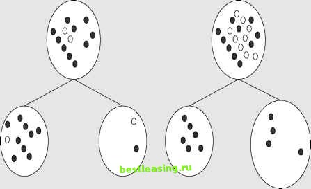

Which of these two proposed splits increases purity the most?

EVALUATING THE TWO SPLITS USING GINI

As explained in the main text, the Gini score for each of the two children in the first proposed split is 0.12 + 0.92 = 0.820. Since the children are the same size, this is also the score for the split.

What about the second proposed split? The Gini score of the left child is 1 since only one class is represented. The Gini score of the right child is

Ginirlght = (4/14) 2 + (10/14) 2 = 0.082 + 0.510 = 0.592

and the Gini score for the split is:

(6/20)Ginileft + (14/20)Giniright = 0.3*1 + 0.7*0.592 = 0.714

Since the Gini score for the first proposed split (0.820) is greater than for the second proposed split (0.714), a tree built using the Gini criterion will prefer the split that yields two nearly pure children over the split that yields one completely pure child along with a larger, less pure one.

(continued)

COMPARING TWO SPLITS USING GINI AND ENTROPY (continued)

EVALUATING THE TWO SPLITS USING ENTROPY

As calculated in the main text, the entropy of the parent node is 1. The entropy of the first proposed split is also calculated in the main text and found to be 0.47 so the information gain for the first proposed split is 0.53.

How much information is gained by the second proposed split? The left child is pure and so has entropy of 0. As for the right child, the formula for entropy is

-(P(dark)log2P(dark) + P(light)log2P(light))

so the entropy of the right child is:

EntropyrlBht = -((4/14)log2(4/14) + (10/14)log2(10/14)) = 0.516 + 0.347 = 0.863

The entropy of the split is the weighted average of the entropies of the resulting nodes. In this case,

0.3*Entropyleft + 0.7*EntropyrlBht = 0.3*0 + 0.7*0.863 = 0.604

Subtracting 0.604 from the entropy of the parent (which is 1) yields an information gain of 0.396. This is less than 0.53, the information gain from the first proposed split, so in this case, entropy splitting criterion also prefers the first split to the second. Compared to Gini, the entropy criterion does have a stronger preference for nodes that are purer, even if smaller. This may be appropriate in domains where there really are clear underlying rules, but it tends to lead to less stable trees in noisy domains such as response to marketing offers.

For example, suppose the target variable is a binary flag indicating whether or not customers continued their subscriptions at the end of the introductory offer period and the proposed split is on acquisition channel, a categorical variable with three classes: direct mail, outbound call, and email. If the acquisition channel had no effect on renewal rate, we would expect the number of renewals in each class to be proportional to the number of customers acquired through that channel. For each channel, the chi-square test subtracts that expected number of renewals from the actual observed renewals, squares the difference, and divides the difference by the expected number. The values for each class are added together to arrive at the score. As described in Chapter 5, the chi-square distribution provide a way to translate this chi-square score into a probability. To measure the purity of a split in a decision tree, the score is sufficient. A high score means that the proposed split successfully splits the population into subpopulations with significantly different distributions.

The chi-square test gives its name to CHAID, a well-known decision tree algorithm first published by John A. Hartigan in 1975. The full acronym stands for Chi-square Automatic Interaction Detector. As the phrase automatic interaction detector implies, the original motivation for CHAID was for detecting

Team-Fly®