statistical relationships between variables. It does this by building a decision tree, so the method has come to be used as a classification tool as well. CHAID makes use of the Chi-square test in several ways-first to merge classes that do not have significantly different effects on the target variable; then to choose a best split; and finally to decide whether it is worth performing any additional splits on a node. In the research community, the current fashion is away from methods that continue splitting only as long as it seems likely to be useful and towards methods that involve pruning. Some researchers, however, still prefer the original CHAID approach, which does not rely on pruning.

The chi-square test applies to categorical variables so in the classic CHAID algorithm, input variables must be categorical. Continuous variables must be binned or replaced with ordinal classes such as high, medium, low. Some current decision tree tools such as SAS Enterprise Miner, use the chi-square test for creating splits using categorical variables, but use another statistical test, the F test, for creating splits on continuous variables. Also, some implementations of CHAID continue to build the tree even when the splits are not statistically significant, and then apply pruning algorithms to prune the tree back.

Reduction in Variance

The four previous measures of purity all apply to categorical targets. When the target variable is numeric, a good split should reduce the variance of the target variable. Recall that variance is a measure of the tendency of the values in a population to stay close to the mean value. In a sample with low variance, most values are quite close to the mean; in a sample with high variance, many values are quite far from the mean. The actual formula for the variance is the mean of the sums of the squared deviations from the mean. Although the reduction in variance split criterion is meant for numeric targets, the dark and light dots in Figure 6.5 can still be used to illustrate it by considering the dark dots to be 1 and the light dots to be 0. The mean value in the parent node is clearly 0.5. Every one of the 20 observations differs from the mean by 0.5, so the variance is (20 * 0.52) / 20 = 0.25. After the split, the left child has 9 dark spots and one light spot, so the node mean is 0.9. Nine of the observations differ from the mean value by 0.1 and one observation differs from the mean value by 0.9 so the variance is (0.92 + 9 * 0.12) / 10 = 0.09. Since both nodes resulting from the split have variance 0.09, the total variance after the split is also 0.09. The reduction in variance due to the split is 0.25 - 0.09 = 0.16.

F Test

Another split criterion that can be used for numeric target variables is the F test, named for another famous Englishman-statistician, astronomer, and geneticist, Ronald. A. Fisher. Fisher and Pearson reportedly did not get along despite, or perhaps because of, the large overlap in their areas of interest. Fishers test

does for continuous variables what Pearsons chi-square test does for categorical variables. It provides a measure of the probability that samples with different means and variances are actually drawn from the same population.

There is a well-understood relationship between the variance of a sample and the variance of the population from which it was drawn. (In fact, so long as the samples are of reasonable size and randomly drawn from the population, sample variance is a good estimate of population variance; very small samples-with fewer than 30 or so observations-usually have higher variance than their corresponding populations.) The F test looks at the relationship between two estimates of the population variance-one derived by pooling all the samples and calculating the variance of the combined sample, and one derived from the between-sample variance calculated as the variance of the sample means. If the various samples are randomly drawn from the same population, these two estimates should agree closely.

The F score is the ratio of the two estimates. It is calculated by dividing the between-sample estimate by the pooled sample estimate. The larger the score, the less likely it is that the samples are all randomly drawn from the same population. In the decision tree context, a large F-score indicates that a proposed split has successfully split the population into subpopulations with significantly different distributions.

Pruning

As previously described, the decision tree keeps growing as long as new splits can be found that improve the ability of the tree to separate the records of the training set into increasingly pure subsets. Such a tree has been optimized for the training set, so eliminating any leaves would only increase the error rate of the tree on the training set. Does this imply that the full tree will also do the best job of classifying new datasets? Certainly not!

A decision tree algorithm makes its best split first, at the root node where there is a large population of records. As the nodes get smaller, idiosyncrasies of the particular training records at a node come to dominate the process. One way to think of this is that the tree finds general patterns at the big nodes and patterns specific to the training set in the smaller nodes; that is, the tree over-fits the training set. The result is an unstable tree that will not make good predictions. The cure is to eliminate the unstable splits by merging smaller leaves through a process called pruning; three general approaches to pruning are discussed in detail.

The CART Pruning Algorithm

CART is a popular decision tree algorithm first published by Leo Breiman, Jerome Friedman, Richard Olshen, and Charles Stone in 1984. The acronym stands for Classification and Regression Trees. The CART algorithm grows binary trees and continues splitting as long as new splits can be found that increase purity. As illustrated in Figure 6.6, inside a complex tree, there are many simpler subtrees, each of which represents a different trade-off between model complexity and training set misclassification rate. The CART algorithm identifies a set of such subtrees as candidate models. These candidate subtrees are applied to the validation set and the tree with the lowest validation set mis-classification rate is selected as the final model.

Creating the Candidate Subtrees

The CART algorithm identifies candidate subtrees through a process of repeated pruning. The goal is to prune first those branches providing the least additional predictive power per leaf. In order to identify these least useful branches, CART relies on a concept called the adjusted error rate. This is a measure that increases each nodes misclassification rate on the training set by imposing a complexity penalty based on the number of leaves in the tree. The adjusted error rate is used to identify weak branches (those whose misclassification rate is not low enough to overcome the penalty) and mark them for pruning.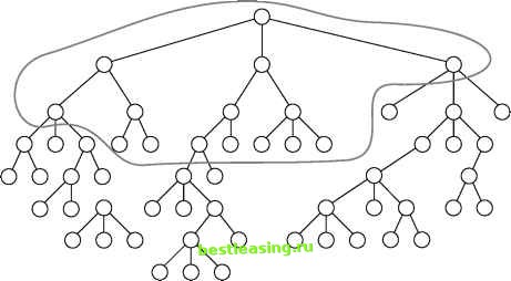

Figure 6.6 Inside a complex tree, there are simpler, more stable trees.