Taking Cost into Account

In the discussion so far, the error rate has been the sole measure for evaluating the fitness of rules and subtrees. In many applications, however, the costs of misclassification vary from class to class. Certainly, in a medical diagnosis, a false negative can be more harmful than a false positive; a scary Pap smear result that, on further investigation, proves to have been a false positive, is much preferable to an undetected cancer. A cost function multiplies the probability of misclassification by a weight indicating the cost of that misclassifica-tion. Several tools allow the use of such a cost function instead of an error function for building decision trees.

Further Refinements to the Decision Tree Method

Although they are not found in most commercial data mining software packages, there are some interesting refinements to the basic decision tree method that are worth discussing.

Using More Than One Field at a Time

Most decision tree algorithms test a single variable to perform each split. This approach can be problematic for several reasons, not least of which is that it can lead to trees with more nodes than necessary. Extra nodes are cause for concern because only the training records that arrive at a given node are available for inducing the subtree below it. The fewer training examples per node, the less stable the resulting model.

Suppose that we are interested in a condition for which both age and gender are important indicators. If the root node split is on age, then each child node contains only about half the women. If the initial split is on gender, then each child node contains only about half the old folks.

Several algorithms have been developed to allow multiple attributes to be used in combination to form the splitter. One technique forms Boolean conjunctions of features in order to reduce the complexity of the tree. After finding the feature that forms the best split, the algorithm looks for the feature which, when combined with the feature chosen first, does the best job of improving the split. Features continue to be added as long as there continues to be a statistically significant improvement in the resulting split.

This procedure can lead to a much more efficient representation of classification rules. As an example, consider the task of classifying the results of a vote according to whether the motion was passed unanimously. For simplicity, consider the case where there are only three votes cast. (The degree of simplification to be made only increases with the number of voters.)

Table 6.1 contains all possible combinations of three votes and an added column to indicate the unanimity of the result.

Table 6.1 All Possible Combinations of Votes by Three Voters

Figure 6.10 shows a tree that perfectly classifies the training data, requiring five internal splitting nodes. Do not worry about how this tree is created, since that is unnecessary to the point we are making.

Allowing features to be combined using the logical and function to form conjunctions yields the much simpler tree in Figure 6.11. The second tree illustrates another potential advantage that can arise from using combinations of fields. The tree now comes much closer to expressing the notion of unanimity that inspired the classes: When all voters agree, the decision is unanimous.

True

Voter #1

Yes No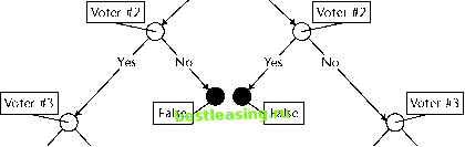

Yes No

False

Yes No

False

True

Figure 6.10 The best binary tree for the unanimity function when splitting on single fields.

Voter #1 and Voter #2 and Voter #3 all vote yes?

s No

Voter #1 and Voter #2 and Voter #3 all vote no?

True

Yes No

True

False

Figure 6.11 Combining features simplifies the tree for defining unanimity.

A tree that can be understood all at once is said, by machine learning researchers, to have good mental fit. Some researchers in the machine learning field attach great importance to this notion, but that seems to be an artifact of the tiny, well-structured problems around which they build their studies. In the real world, if a classification task is so simple that you can get your mind around the entire decision tree that represents it, you probably dont need to waste your time with powerful data mining tools to discover it. We believe that the ability to understand the rule that leads to any particular leaf is very important; on the other hand, the ability to interpret an entire decision tree at a glance is neither important nor likely to be possible outside of the laboratory.

Tilting the Hyperplane

Classification problems are sometimes presented in geometric terms. This way of thinking is especially natural for datasets having continuous variables for all fields. In this interpretation, each record is a point in a multidimensional space. Each field represents the position of the record along one axis of the space. Decision trees are a way of carving the space into regions, each of which is labeled with a class. Any new record that falls into one of the regions is classified accordingly.

Traditional decision trees, which test the value of a single field at each node, can only form rectangular regions. In a two-dimensional space, a test of the form Y less than some constant forms a region bounded by a line perpendicular to the Y-axis and parallel to the X-axis. Different values for the constant cause the line to move up and down, but the line remains horizontal. Similarly, in a space of higher dimensionality, a test on a single field defines a hyperplane that is perpendicular to the axis represented by the field used in the test and parallel to all the other axes. In a two-dimensional space, with only horizontal and vertical lines to work with, the resulting regions are rectangular. In three-dimensional