

|
|

|
Промышленный лизинг
Методички
part of the target class. Figure 6.14 illustrates this point using two species of dinosaur. The decision tree (represented as a box diagram) has successfully isolated the stegosaurs from the triceratops. In the credit card industry, for example, there are several ways for customers to be profitable. Some profitable customers have low transaction rates, but keep high revolving balances without defaulting. Others pay off their balance in full each month, but are profitable due to the high transaction volume they generate. Yet others have few transactions, but occasionally make a large purchase and take several months to pay it off. Two very dissimilar customers may be equally profitable. A decision tree can find each separate group, label it, and by providing a description of the box itself, suggest the reason for each groups profitability. Tree Ring Diagrams Another clever representation of a decision tree is used by the Enterprise Miner product from SAS Institute. The diagram in Figure 6.15 looks as though the tree has been cut down and we are looking at the stump. 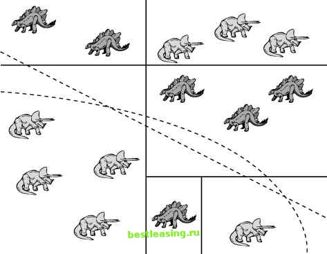 Figure 6.14 Often a simple line or curve cannot separate the regions and a decision tree does better. 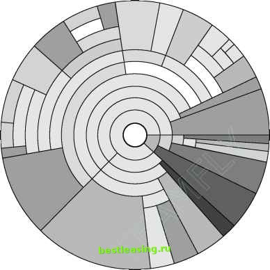 Figure 6.15 A tree ring diagram produced by SAS Enterprise Miner summarizes the different levels of the tree. The circle at the center of the diagram represents the root node, before any splits have been made. Moving out from the center, each concentric ring represents a new level in the tree. The ring closest to the center represents the root node split. The arc length is proportional to the number of records taking each of the two paths, and the shading represents the nodes purity. The first split in the model represented by this diagram is fairly unbalanced. It divides the records into two groups, a large one where the concentration is little different from the parent population, and a small one with a high concentration of the target class. At the next level, this smaller node is again split and one branch, represented by the thin, dark pie slice that extends all the way through to the outermost ring of the diagram, is a leaf node. The ring diagram shows the trees depth and complexity at a glance and indicates the location of high concentrations on the target class. What it does not show directly are the rules defining the nodes. The software reveals these when a user clicks on a particular section of the diagram. Team-Fly® Decision Trees in Practice Decision trees can be applied in many different situations. To explore a large dataset to pick out useful variables To predict future states of important variables in an industrial process To form directed clusters of customers for a recommendation system This section includes examples of decision trees being used in all of these ways. Decision Trees as a Data Exploration Tool During the data exploration phase of a data mining project, decision trees are a useful tool for picking the variables that are likely to be important for predicting particular targets. One of our newspaper clients, The Boston Globe, was interested in estimating a towns expected home delivery circulation level based on various demographic and geographic characteristics. Armed with such estimates, they would, among other things, be able to spot towns with untapped potential where the actual circulation was lower than the expected circulation. The final model would be a regression equation based on a handful of variables. But which variables? And what exactly would the regression attempt to estimate? Before building the regression model, we used decision trees to help explore these questions. Although the newspaper was ultimately interested in predicting the actual number of subscribing households in a given city or town, that number does not make a good target for a regression model because towns and cities vary so much in size. It is not useful to waste modeling power on discovering that there are more subscribers in large towns than in small ones. A better target is the penetration-the proportion of households that subscribe to the paper. This number yields an estimate of the total number of subscribing households simply by multiply it by the number of households in a town. Factoring out town size yields a target variable with values that range from zero to somewhat less than one. The next step was to figure out which factors, from among the hundreds in the town signature, separate towns with high penetration (the good towns) from those with low penetration (the bad towns). Our approach was to build decision tree with a binary good/bad target variable. This involved sorting the towns by home delivery penetration and labeling the top one third good and the bottom one third bad. Towns in the middle third-those that are not clearly good or bad-were left out of the training set. The screen shot in Figure 6.16 shows the top few levels of one of the resulting trees. 1 2 3 4 5 6 7 8 9 10 11 12 13 14 15 16 17 18 19 20 21 22 23 24 25 26 27 28 29 30 31 32 33 34 35 36 37 38 39 40 41 42 43 44 45 46 47 48 49 50 51 52 53 54 55 56 57 58 59 60 61 62 63 64 65 66 67 68 69 70 71 72 73 74 [ 75 ] 76 77 78 79 80 81 82 83 84 85 86 87 88 89 90 91 92 93 94 95 96 97 98 99 100 101 102 103 104 105 106 107 108 109 110 111 112 113 114 115 116 117 118 119 120 121 122 123 124 125 126 127 128 129 130 131 132 133 134 135 136 137 138 139 140 141 142 143 144 145 146 147 148 149 150 151 152 153 154 155 156 157 158 159 160 161 162 163 164 165 166 167 168 169 170 171 172 173 174 175 176 177 178 179 180 181 182 183 184 185 186 187 188 189 190 191 192 193 194 195 196 197 198 199 200 201 202 203 204 205 206 207 208 209 210 211 212 213 214 215 216 217 218 219 220 221 222 |