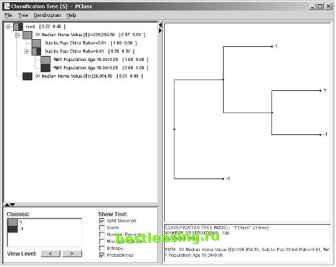Figure 6.16 A decision tree separates good towns from the bad, as visualized by Insightful Miner.

The tree shows that median home value is the best first split. Towns where the median home value (in a region with some of the most expensive housing in the country) is less than $226,000 dollars are poor prospects for this paper. The split at the next level is more surprising. The variable chosen for the split is one of a family of derived variables comparing the subscriber base in the town to the town population as a whole. Towns where the subscribers are similar to the general population are better, in terms of home delivery penetration, than towns where the subscribers are farther from the mean. Other variables that were important for distinguishing good from bad towns included the mean years of school completed, the percentage of the population in blue collar occupations, and the percentage of the population in high-status occupations. All of these ended up as inputs to the regression model.

Some other variables that we had expected to be important such as distance from Boston and household income turned out to be less powerful. Once the decision tree has thrown a spotlight on a variable by either including it or failing to use it, the reason often becomes clear with a little thought. The problem with distance from Boston, for instance, is that as one first drives out into the suburbs, home penetration goes up with distance from Boston. After a while, however, distance from Boston becomes negatively correlated with penetration as people far from Boston do not care as much about what goes on there. Home price is a better predictor because its distribution resembles that of the target variable, increasing in the first few miles and then declining. The decision tree provides guidance about which variables to think about as well as which variables to use.

Applying Decision-Tree Methods to Sequential Events

Predicting the future is one of the most important applications of data mining. The task of analyzing trends in historical data in order to predict future behavior recurs in every domain we have examined.

One of our clients, a major bank, looked at the detailed transaction data from its customers in order to spot earlier warning signs for attrition in its checking accounts. ATM withdrawals, payroll-direct deposits, balance inquiries, visits to the teller, and hundreds of other transaction types and customer attributes were tracked over time to find signatures that allow the bank to recognize that a customers loyalty is beginning to weaken while there is still time to take corrective action.

Another client, a manufacturer of diesel engines, used the decision tree component of SPSSs Clementine data mining suite to forecast diesel engine sales based on historical truck registration data. The goal was to identify individual owner-operators who were likely to be ready to trade in the engines of their big rigs.

Sales, profits, failure modes, fashion trends, commodity prices, operating temperatures, interest rates, call volumes, response rates, and return rates: People are trying to predict them all. In some fields, notably economics, the analysis of time-series data is a central preoccupation of statistical analysts, so you might expect there to be a large collection of ready-made techniques available to be applied to predictive data mining on time-ordered data. Unfortunately, this is not the case.

For one thing, much of the time-series analysis work in other fields focuses on analyzing patterns in a single variable such as the dollar-yen exchange rate or unemployment in isolation. Corporate data warehouses may well contain data that exhibits cyclical patterns. Certainly, average daily balances in checking accounts reflect that rents are typically due on the first of the month and that many people are paid on Fridays, but, for the most part, these sorts of patterns are not of interest because they are neither unexpected nor actionable.

In commercial data mining, our focus is on how a large number of independent variables combine to predict some future outcome. Chapter 9 discusses how time can be integrated into association rules in order to find sequential patterns. Decision-tree methods have also been applied very successfully in this domain, but it is generally necessary to enrich the data with trend information by including fields such as differences and rates of change that explicitly represent change over time. Chapter 17 discusses these data preparation issues in more detail. The following section describes an application that automatically generates these derived fields and uses them to build a tree-based simulator that can be used to project an entire database into the future.

Simulating the Future

This discussion is largely based on discussions with Marc Goodman and on his 1995 doctoral dissertation on a technique called projective visualization. Pro-jective visualization uses a database of snapshots of historical data to develop a simulator. The simulation can be run to project the values of all variables into the future. The result is an extended database whose new records have exactly the same fields as the original, but with values supplied by the simulator rather than by observation. The approach is described in more detail in the technical aside.

Case Study: Process Control in a Coffee-Roasting Plant

Nestle, one of the largest food and beverages companies in the world, used a number of continuous-feed coffee roasters to produce a variety of coffee products including Nescafe Granules, Gold Blend, Gold Blend Decaf, and Blend 37. Each of these products has a recipe that specifies target values for a plethora of roaster variables such as the temperature of the air at various exhaust points, the speed of various fans, the rate that gas is burned, the amount of water introduced to quench the beans, and the positions of various flaps and valves. There are a lot of ways for things to go wrong when roasting coffee, ranging from a roast coming out too light in color to a costly and damaging roaster fire. A bad batch of roasted coffee incurs a big cost; damage to equipment is even more expensive.

To help operators keep the roaster running properly, data is collected from about 60 sensors. Every 30 seconds, this data, along with control information, is written to a log and made available to operators in the form of graphs. The project described here took place at a Nestle research laboratory in York, England. Nestle used projective visualization to build a coffee roaster simulation based on the sensor logs.

Goals for the Simulator

Nestle saw several ways that a coffee roaster simulator could improve its processes.

By using the simulator to try out new recipes, a large number of new recipes could be evaluated without interrupting production. Furthermore, recipes that might lead to roaster fires or other damage could be eliminated in advance.

The simulator could be used to train new operators and expose them to routine problems and their solutions. Using the simulator, operators could try out different approaches to resolving a problem.