USING DECISION TREES FOR PROJECTIVE VISUALIZATION

Using Goodmans terminology, which comes from the machine learning field, each snapshot of a moment in time is called a case. A case is made up of attributes, which are the fields in the case record. Attributes may be of any data type and may be continuous or categorical. The attributes are used to form features. Features are Boolean (yes/no) variables that are combined in various ways to form the internal nodes of a decision tree. For example, if the database contains a numeric salary field, a continuous attribute, then that might lead to creation of a feature such as salary < 38,500.

For a continuous variable like salary, a feature of the form attribute < value is generated for every value observed in the training set. This means that there are potentially as many features derived from an attribute as there are cases in the training set. Features based on equality or set membership are generated for symbolic attributes and literal attributes such as names of people or places.

The attributes are also used to generate interpretations; these are new attributes derived from the given ones. Interpretations generally reflect knowledge of the domain and what sorts of relationships are likely to be important. In the current problem, finding patterns that occur over time, the amount, direction, and rate of change in the value of an attribute from one time period to the next are likely to be important. Therefore, for each numeric attribute, the software automatically generates interpretations for the difference and the discrete first and second derivatives of the attribute.

In general, however, the user supplies interpretations. For example, in a credit risk model, it is likely that the ratio of debt to income is more predictive than the magnitude of either. With this knowledge we might add an interpretation that was the ratio of those two attributes. Often, user-supplied interpretations combine attributes in ways that the program would not come up with automatically. Examples include calculating a great-circle distance from changes in latitude and longitude or taking the product of three linear measurements to get a volume.

FROM ONE CASE TO THE NEXT

The central idea behind projective visualization is to use the historical cases to generate a set of rules for generating case n+1 from case n. When this model is applied to the final observed case, it generates a new projected case. To project more than one time step into the future, we continue to apply the model to the most recently created case. Naturally, confidence in the projected values decreases as the simulation is run for more and more time steps.

The figure illustrates the way a single attribute is projected using a decision tree based on the features generated from all the other attributes and interpretations in the previous case. During the training process, a separate decision tree is grown for each attribute. This entire forest is evaluated in order to move from one simulation step to the next.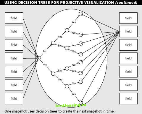

The simulator could track the operation of the actual roaster and project it several minutes into the future. When the simulation ran into a problem, an alert could be generated while the operators still had time to avert trouble.

Evaluation of the Roaster Simulation

The simulation was built using a training set of 34,000 cases. The simulation was then evaluated using a test set of around 40,000 additional cases that had not been part of the training set. For each case in the test set, the simulator generated projected snapshots 60 steps into the future. At each step the projected values of all variables were compared against the actual values. As expected, the size of the error increases with time. For example, the error rate for product temperature turned out to be 2/3°C per minute of projection, but even 30 minutes into the future the simulator is doing considerably better than random guessing.

The roaster simulator turned out to be more accurate than all but the most experienced operators at projecting trends, and even the most experienced operators were able to do a better job with the aid of the simulator. Operators

enjoyed using the simulator and reported that it gave them new insight into corrective actions.

Lessons Learned

Decision-tree methods have wide applicability for data exploration, classification, and scoring. They can also be used for estimating continuous values although they are rarely the first choice since decision trees generate lumpy estimates-all records reaching the same leaf are assigned the same estimated value. They are a good choice when the data mining task is classification of records or prediction of discrete outcomes. Use decision trees when your goal is to assign each record to one of a few broad categories. Theoretically, decision trees can assign records to an arbitrary number of classes, but they are error-prone when the number of training examples per class gets small. This can happen rather quickly in a tree with many levels and/or many branches per node. In many business contexts, problems naturally resolve to a binary classification such as responder/nonresponder or good/bad so this is not a large problem in practice.

Decision trees are also a natural choice when the goal is to generate understandable and explainable rules. The ability of decision trees to generate rules that can be translated into comprehensible natural language or SQL is one of the greatest strengths of the technique. Even in complex decision trees , it is generally fairly easy to follow any one path through the tree to a particular leaf. So the explanation for any particular classification or prediction is relatively straightforward.

Decision trees require less data preparation than many other techniques because they are equally adept at handling continuous and categorical variables. Categorical variables, which pose problems for neural networks and statistical techniques, are split by forming groups of classes. Continuous variables are split by dividing their range of values. Because decision trees do not make use of the actual values of numeric variables, they are not sensitive to outliers and skewed distributions. This robustness comes at the cost of throwing away some of the information that is available in the training data, so a well-tuned neural network or regression model will often make better use of the same fields than a decision tree. For that reason, decision trees are often used to pick a good set of variables to be used as inputs to another modeling technique. Time-oriented data does require a lot of data preparation. Time series data must be enhanced so that trends and sequential patterns are made visible.

Decision trees reveal so much about the data to which they are applied that the authors make use of them in the early phases of nearly every data mining project even when the final models are to be created using some other technique.