

|
|

|
Промышленный лизинг
Методички
Feed-forward networks are the simplest and most useful type of network for directed modeling. There are three basic questions to ask about them: What are units and how do they behave? That is, what is the activation function? How are the units connected together? That is, what is the topology of a network? How does the network learn to recognize patterns? That is, what is back propagation and more generally how is the network trained? The answers to these questions provide the background for understanding basic neural networks, an understanding that provides guidance for getting the best results from this powerful data mining technique. What Is the Unit of a Neural Network? Figure 7.4 shows the important features of the artificial neuron. The unit combines its inputs into a single value, which it then transforms to produce the output; these together are called the activation function. The most common activation functions are based on the biological model where the output remains very low until the combined inputs reach a threshold value. When the combined inputs reach the threshold, the unit is activated and the output is high. Like its biological counterpart, the unit in a neural network has the property that small changes in the inputs, when the combined values are within some middle range, can have relatively large effects on the output. Conversely, large changes in the inputs may have little effect on the output, when the combined inputs are far from the middle range. This property, where sometimes small changes matter and sometimes they do not, is an example of nonlinear behavior. The power and complexity of neural networks arise from their nonlinear behavior, which in turn arises from the particular activation function used by the constituent neural units. The activation function has two parts. The first part is the combination function that merges all the inputs into a single value. As shown in Figure 7.4, each input into the unit has its own weight. The most common combination function is the weighted sum, where each input is multiplied by its weight and these products are added together. Other combination functions are sometimes useful and include the maximum of the weighted inputs, the minimum, and the logical AND or OR of the values. Although there is a lot of flexibility in the choice of combination functions, the standard weighted sum works well in many situations. This element of choice is a common trait of neural networks. Their basic structure is quite flexible, but the defaults that correspond to the original biological models, such as the weighted sum for the combination function, work well in practice. Team-Fly® The combination the activation I function. 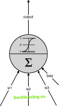 The result is one output value, usually between -1 and 1. The transfer function calculates the output value from the result of the combination function. The combination function combines all the inputs into a single value, usually as a weighted summation. Each input has its own weight, plus there is an additional weight called the bias. inputs Figure 7.4 The unit of an artificial neural network is modeled on the biological neuron. The output of the unit is a nonlinear combination of its inputs. The second part of the activation function is the transfer function, which gets its name from the fact that it transfers the value of the combination function to the output of the unit. Figure 7.5 compares three typical transfer functions: the sigmoid (logistic), linear, and hyperbolic tangent functions. The specific values that the transfer function takes on are not as important as the general form of the function. From our perspective, the linear transfer function is the least interesting. A feed-forward neural network consisting only of units with linear transfer functions and a weighted sum combination function is really just doing a linear regression. Sigmoid functions are S-shaped functions, of which the two most common for neural networks are the logistic and the hyperbolic tangent. The major difference between them is the range of their outputs, between 0 and 1 for the logistic and between -1 and 1 for the hyperbolic tangent. The logistic and hyperbolic tangent transfer functions behave in a similar way. Even though they are not linear, their behavior is appealing to statisticians. When the weighted sum of all the inputs is near 0, then these functions are a close approximation of a linear function. Statisticians appreciate linear systems, and almost-linear systems are almost as well appreciated. As the magnitude of the weighted sum gets larger, these transfer functions gradually saturate (to 0 and 1 in the case of the logistic; to -1 and 1 in the case of the hyperbolic tangent). This behavior corresponds to a gradual movement from a linear model of the input to a nonlinear model. In short, neural networks have the ability to do a good job of modeling on three types of problems: linear problems, near-linear problems, and nonlinear problems. There is also a relationship between the activation function and the range of input values, as discussed in the sidebar, Sigmoid Functions and Ranges for Input Values. A network can contain units with different transfer functions, a subject well return to later when discussing network topology. Sophisticated tools sometimes allow experimentation with other combination and transfer functions. Other functions have significantly different behavior from the standard units. It may be fun and even helpful to play with different types of activation functions. If you do not want to bother, though, you can have confidence in the standard functions that have proven successful for many neural network applications. -0.5 -1.0 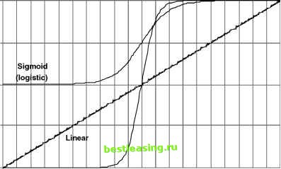 Exponential (tanh) 0 Figure 7.5 Three common transfer functions are the sigmoid, linear, and hyperbolic tangent functions. 1 2 3 4 5 6 7 8 9 10 11 12 13 14 15 16 17 18 19 20 21 22 23 24 25 26 27 28 29 30 31 32 33 34 35 36 37 38 39 40 41 42 43 44 45 46 47 48 49 50 51 52 53 54 55 56 57 58 59 60 61 62 63 64 65 66 67 68 69 70 71 72 73 74 75 76 77 78 79 80 81 [ 82 ] 83 84 85 86 87 88 89 90 91 92 93 94 95 96 97 98 99 100 101 102 103 104 105 106 107 108 109 110 111 112 113 114 115 116 117 118 119 120 121 122 123 124 125 126 127 128 129 130 131 132 133 134 135 136 137 138 139 140 141 142 143 144 145 146 147 148 149 150 151 152 153 154 155 156 157 158 159 160 161 162 163 164 165 166 167 168 169 170 171 172 173 174 175 176 177 178 179 180 181 182 183 184 185 186 187 188 189 190 191 192 193 194 195 196 197 198 199 200 201 202 203 204 205 206 207 208 209 210 211 212 213 214 215 216 217 218 219 220 221 222 |