SIGMOID FUNCTIONS AND RANGES FOR INPUT VALUES

The sigmoid activation functions are S-shaped curves that fall within bounds. For instance, the logistic function produces values between 0 and 1, and the hyperbolic tangent produces values between -1 and 1 for all possible outputs of the summation function. The formulas for these functions are:

logistic(x) = 1/(1 + e-x)

tanh(x) = (ex- ex)/(ex + e-x)

When used in a neural network, the x is the result of the combination function, typically the weighted sum of the inputs into the unit.

Since these functions are defined for all values of x, why do we recommend that the inputs to a network be in a small range, typically from -1 to 1? The reason has to do with how these functions behave near 0. In this range, they behave in an almost linear way. That is, small changes in x result in small changes in the output; changing x by half as much results in about half the effect on the output. The relationship is not exact, but it is a close approximation.

For training purposes, it is a good idea to start out in this quasi-linear area. As the neural network trains, nodes may find linear relationships in the data. These nodes adjust their weights so the resulting value falls in this linear range. Other nodes may find nonlinear relationships. Their adjusted weights are likely to fall in a larger range.

Requiring that all inputs be in the same range also prevents one set of inputs, such as the price of a house-a big number in the tens of thousands- from dominating other inputs, such as the number of bedrooms. After all, the combination function is a weighted sum of the inputs, and when some values are very large, they will dominate the weighted sum. When x is large, small adjustments to the weights on the inputs have almost no effect on the output of the unit making it difficult to train. That is, the sigmoid function can take advantage of the difference between one and two bedrooms, but a house that costs $50,000 and one that costs $1,000,000 would be hard for it to distinguish, and it can take many generations of training the network for the weights associated with this feature to adjust. Keeping the inputs relatively small enables adjustments to the weights to have a bigger impact. This aid to training is the strongest reason for insisting that inputs stay in a small range.

In fact, even when a feature naturally falls into a range smaller than -1 to 1, such as 0.5 to 0.75, it is desirable to scale the feature so the input to the network uses the entire range from -1 to 1. Using the full range of values from -1 to 1 ensures the best results.

Although we recommend that inputs be in the range from -1 to 1, this should be taken as a guideline, not a strict rule. For instance, standardizing variables-subtracting the mean and dividing by the standard deviation-is a common transformation on variables. This results in small enough values to be useful for neural networks.

Feed-Forward Neural Networks

A feed-forward neural network calculates output values from input values, as shown in Figure 7.6. The topology, or structure, of this network is typical of networks used for prediction and classification. The units are organized into three layers. The layer on the left is connected to the inputs and called the input layer. Each unit in the input layer is connected to exactly one source field, which has typically been mapped to the range -1 to 1. In this example, the input layer does not actually do any work. Each input layer unit copies its input value to its output. If this is the case, why do we even bother to mention it here? It is an important part of the vocabulary of neural networks. In practical terms, the input layer represents the process for mapping values into a reasonable range. For this reason alone, it is worth including them, because they are a reminder of a very important aspect of using neural networks successfully.

output from unit

input weight

constant input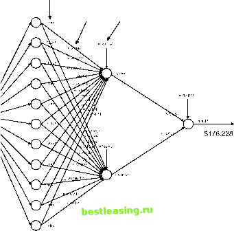

Figure 7.6 The real estate training example shown here provides the input into a feedforward neural network and illustrates that a network is filled with seemingly meaningless weights.

The next layer is called the hidden layer because it is connected neither to the inputs nor to the output of the network. Each unit in the hidden layer is typically fully connected to all the units in the input layer. Since this network contains standard units, the units in the hidden layer calculate their output by multiplying the value of each input by its corresponding weight, adding these up, and applying the transfer function. A neural network can have any number of hidden layers, but in general, one hidden layer is sufficient. The wider the layer (that is, the more units it contains) the greater the capacity of the network to recognize patterns. This greater capacity has a drawback, though, because the neural network can memorize patterns-of-one in the training examples. We want the network to generalize on the training set, not to memorize it. To achieve this, the hidden layer should not be too wide.

Notice that the units in Figure 7.6 each have an additional input coming down from the top. This is the constant input, sometimes called a bias, and is always set to 1. Like other inputs, it has a weight and is included in the combination function. The bias acts as a global offset that helps the network better understand patterns. The training phase adjusts the weights on constant inputs just as it does on the other weights in the network.

The last unit on the right is the output layer because it is connected to the output of the neural network. It is fully connected to all the units in the hidden layer. Most of the time, the neural network is being used to calculate a single value, so there is only one unit in the output layer and the value. We must map this value back to understand the output. For the network in Figure 7.6, we have to convert 0.49815 back into a value between $103,000 and $250,000. It corresponds to $176,228, which is quite close to the actual value of $171,000. In some implementations, the output layer uses a simple linear transfer function, so the output is a weighted linear combination of inputs. This eliminates the need to map the outputs.

It is possible for the output layer to have more than one unit. For instance, a department store chain wants to predict the likelihood that customers will be purchasing products from various departments, such as womens apparel, furniture, and entertainment. The stores want to use this information to plan promotions and direct target mailings.

To make this prediction, they might set up the neural network shown in Figure 7.7. This network has three outputs, one for each department. The outputs are a propensity for the customer described in the inputs to make his or her next purchase from the associated department.