propensity to purchase

womens apparel

propensity to purchase

furniture

propensity to purchase

entertainment

Figure 7.7 This network has with more than one output and is used to predict the department where department store customers will make their next purchase.

After feeding the inputs for a customer into the network, the network calculates three values. Given all these outputs, how can the department store determine the right promotion or promotions to offer the customer? Some common methods used when working with multiple model outputs are:

Take the department corresponding to the output with the maximum value.

Take departments corresponding to the outputs with the top three values.

Take all departments corresponding to the outputs that exceed some threshold value.

Take all departments corresponding to units that are some percentage of the unit with the maximum value.

All of these possibilities work well and have their strengths and weaknesses in different situations. There is no one right answer that always works. In practice, you want to try several of these possibilities on the test set in order to determine which works best in a particular situation.

There are other variations on the topology of feed-forward neural networks. Sometimes, the input layers are connected directly to the output layer. In this case, the network has two components. These direct connections behave like a standard regression (linear or logistic, depending on the activation function in the output layer). This is useful building more standard statistical models. The hidden layer then acts as an adjustment to the statistical model.

How Does a Neural Network Learn Using Back Propagation?

Training a neural network is the process of setting the best weights on the edges connecting all the units in the network. The goal is to use the training set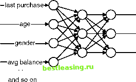

to calculate weights where the output of the network is as close to the desired output as possible for as many of the examples in the training set as possible. Although back propagation is no longer the preferred method for adjusting the weights, it provides insight into how training works and it was the original method for training feed-forward networks. At the heart of back propagation are the following three steps:

1. The network gets a training example and, using the existing weights in the network, it calculates the output or outputs.

2. Back propagation then calculates the error by taking the difference between the calculated result and the expected (actual result).

3. The error is fed back through the network and the weights are adjusted to minimize the error-hence the name back propagation because the errors are sent back through the network.

The back propagation algorithm measures the overall error of the network by comparing the values produced on each training example to the actual value. It then adjusts the weights of the output layer to reduce, but not eliminate, the error. However, the algorithm has not finished. It then assigns the blame to earlier nodes the network and adjusts the weights connecting those nodes, further reducing overall error. The specific mechanism for assigning blame is not important. Suffice it to say that back propagation uses a complicated mathematical procedure that requires taking partial derivatives of the activation function.

Given the error, how does a unit adjust its weights? It estimates whether changing the weight on each input would increase or decrease the error. The unit then adjusts each weight to reduce, but not eliminate, the error. The adjustments for each example in the training set slowly nudge the weights, toward their optimal values. Remember, the goal is to generalize and identify patterns in the input, not to memorize the training set. Adjusting the weights is like a leisurely walk instead of a mad-dash sprint. After being shown enough training examples during enough generations, the weights on the network no longer change significantly and the error no longer decreases. This is the point where training stops; the network has learned to recognize patterns in the input.

This technique for adjusting the weights is called the generalized delta rule. There are two important parameters associated with using the generalized delta rule. The first is momentum, which refers to the tendency of the weights inside each unit to change the direction they are heading in. That is, each weight remembers if it has been getting bigger or smaller, and momentum tries to keep it going in the same direction. A network with high momentum responds slowly to new training examples that want to reverse the weights. If momentum is low, then the weights are allowed to oscillate more freely.

TRAINING AS OPTIMIZATION

Although the first practical algorithm for training networks, back propagation is an inefficient way to train networks. The goal of training is to find the set of weights that minimizes the error on the training and/or validation set. This type of problem is an optimization problem, and there are several different approaches.

It is worth noting that this is a hard problem. First, there are many weights in the network, so there are many, many different possibilities of weights to consider. For a network that has 28 weights (say seven inputs and three hidden nodes in the hidden layer). Trying every combination of just two values for each weight requires testing 2Л28 combinations of values-or over 250 million combinations. Trying out all combinations of 10 values for each weight would be prohibitively expensive.

A second problem is one of symmetry. In general, there is no single best value. In fact, with neural networks that have more than one unit in the hidden layer, there are always multiple optima-because the weights on one hidden unit could be entirely swapped with the weights on another. This problem of having multiple optima complicates finding the best solution.

One approach to finding optima is called hill climbing. Start with a random set of weights. Then, consider taking a single step in each direction by making a small change in each of the weights. Choose whichever small step does the best job of reducing the error and repeat the process. This is like finding the highest point somewhere by only taking steps uphill. In many cases, you end up on top of a small hill instead of a tall mountain.

One variation on hill climbing is to start with big steps and gradually reduce the step size (the Jolly Green Giant will do a better job of finding the top of the nearest mountain than an ant). A related algorithm, called simulated annealing, injects a bit of randomness in the hill climbing. The randomness is based on physical theories having to do with how crystals form when liquids cool into solids (the crystalline formation is an example of optimization in the physical world). Both simulated annealing and hill climbing require many, many iterations-and these iterations are expensive computationally because they require running a network on the entire training set and then repeating again, and again for each step.

A better algorithm for training is the conjugate gradient algorithm. This algorithm tests a few different sets of weights and then guesses where the optimum is, using some ideas from multidimensional geometry. Each set of weights is considered to be a single point in a multidimensional space. After trying several different sets, the algorithm fits a multidimensional parabola to the points. A parabola is a U-shaped curve that has a single minimum (or maximum). Conjugate gradient then continues with a new set of weights in this region. This process still needs to be repeated; however, conjugate gradient produces better values more quickly than back propagation or the various hill climbing methods. Conjugate gradient (or some variation of it) is the preferred method of training neural networks in most data mining tools.