can prevent a network from effectively using an important field. Skewed distributions affect neural networks but not decision trees because neural networks actually use the values for calculations; decision trees only use the ordering (rank) of the values.

There are several ways to resolve this. The most common is to split a feature like income into ranges. This is called discretizing or binning the field. Figure 7.9 illustrates breaking the incomes into 10 equal-width ranges, but this is not useful at all. Virtually all the values fall in the first two ranges. Equal-sized quin-tiles provide a better choice of ranges:

$10,000-$17,999 very low (-1.0) $18,000-$31,999 low (-0.5) $32,000-$63,999 middle (0.0) $64,000-$99,999 high (+0.5) $100,000 and above very high (+1.0)

Information is being lost by this transformation. A household with an income of $65,000 now looks exactly like a household with an income of $98,000. On the other hand, the sheer magnitude of the larger values does not confuse the neural network.

There are other methods as well. For instance, taking the logarithm is a good way of handling values that have wide ranges. Another approach is to standardize the variable, by subtracting the mean and dividing by the standard deviation. The standardized value is going to very often be between -2 and +2 (that is, for most variables, almost all values fall within two standard deviations of the mean). Standardizing variables is often a good approach for neural networks. However, it must be used with care, since big outliers make the standard deviation big. So, when there are big outliers, many of the standardized values will fall into a very small range, making it hard for the network to distinguish them from each other.

40,000 35,000 30,000 25,000 20,000 15,000 10,000 5,000 0

region 1

region

region 3

region 4

region 5

region 6

region 7

region 8

region 9

region 10

0 $100,000 $200,000 $300,000 $400,000 $500,000 $600,000 $700,000 $800,000 $900,000 $1,000,000

income

Figure 7.9 Household income provides an example of a skewed distribution. Almost all the values are in the first 10 percent of the range (income of less than $100,000).

Features with Ordered, Discrete (Integer) Values

Continuous features can be binned into ordered, discrete values. Other examples of features with ordered values include:

Counts (number of children, number of items purchased, months since sale, and so on)

Age

Ordered categories (low, medium, high)

Like the continuous features, these have a maximum and minimum value. For instance, age usually ranges from 0 to about 100, but the exact range may depend on the data used. The number of children may go from 0 to 4, with anything over 4 considered to be 4. Preparing such fields is simple. First, count the number of different values and assign each a proportional fraction in some range, say from 0 to 1. For instance, if there are five distinct values, then these get mapped to 0, 0.25, 0.50, 0.75, and 1, as shown in Figure 7.10. Notice that mapping the values onto the unit interval like this preserves the ordering; this is an important aspect of this method and means that information is not being lost.

It is also possible to break a range into unequal parts. One example is called thermometer codes:

0 - 0 0 0 0 = 0/16 = 0.0000

1 - 1 0 0 0 = 8/16 = 0.5000

2 - 1 1 0 0 = 12/16 = 0.7500

3 - 1 1 1 0 = 14/16 = 0.8750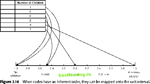

The name arises because the sequence of 1s starts on one side and rises to some value, like the mercury in a thermometer; this sequence is then interpreted as a decimal written in binary notation. Thermometer codes are good for things like academic grades and bond ratings, where the difference on one end of the scale is less significant than differences on the other end.

For instance, for many marketing applications, having no children is quite different from having one child. However, the difference between three children and four is rather negligible. Using a thermometer code, the number of children variable might be mapped as follows: 0 (for 0 children), 0.5 (for one child), 0.75 (for two children), 0.875 (for three children), and so on. For categorical variables, it is often easier to keep mapped values in the range from 0 to 1. This is reasonable. However, to extend the range from -1 to 1, double the value and subtract 1.

Thermometer codes are one way of including prior information into the coding scheme. They keep certain codes values close together because you have a sense that these code values should be close. This type of knowledge can improve the results from a neural network-dont make it discover what you already know. Feel free to map values onto the unit interval so that codes close to each other match your intuitive notions of how close they should be.

Features with Categorical Values

Features with categories are unordered lists of values. These are different from ordered lists, because there is no ordering to preserve and introducing an order is inappropriate. There are typically many examples of categorical values in data, such as:

Gender, marital status

Status codes

Product codes

Zip codes

Although zip codes look like numbers in the United States, they really represent discrete geographic areas, and the codes themselves give little geographic information. There is no reason to think that 10014 is more like 02116 than it is like 94117, even though the numbers are much closer. The numbers are just discrete names attached to geographical areas.

There are three fundamentally different ways of handling categorical features. The first is to treat the codes as discrete, ordered values, mapping them using the methods discussed in the previous section. Unfortunately, the neural network does not understand that the codes are unordered. So, five codes for marital status ( single, divorced, married, widowed, and unknown ) would