The approach is similar when there are more than two options under consideration. For example, consider a long distance carrier trying to target a new set of customers with three targeted service offerings:

Discounts on all international calls

Discounts on all long-distance calls that are not international

Discounts on calls to a predefined set of customers

The carrier is going to offer incentives to customers for each of the three packages. Since the incentives are expensive, the carrier needs to choose the right service for the right customers in order for the campaign to be profitable. Offering all three products to all the customers is expensive and, even worse, may confuse the recipients, reducing the response rate.

The carrier test markets the products to a small subset of customers who receive all three offers but are only allowed to respond to one of them. It intends to use this information to build a model for predicting customer affinity for each offer. The training set uses the data collected from the test marketing campaign, and codes the propensity as follows: no response - -1.00, international - -0.33, national - +0.33, and specific numbers - +1.00. After training a neural network with information about the customers, the carrier starts applying the model.

But, applying the model does not go as well as planned. Many customers cluster around the four values used for training the network. However, apart from the nonresponders (who are the majority), there are many instances when the network returns intermediate values like 0.0 and 0.5. What can be done?

First, the carrier should use a validation set to understand the output values. By interpreting the results of the network based on what happens in the validation set, it can find the right ranges to use for transforming the results of the network back into marketing segments. This is the same process shown in Figure 7.11.

Another observation in this case is that the network is really being used to predict three different things, whether a recipient will respond to each of the campaigns. This strongly suggests that a better structure for the network is to have three outputs: a propensity to respond to the international plan, to the long-distance plan, and to the specific numbers plan. The test set would then be used to determine where the cutoff is for nonrespondents. Alternatively, each outcome could be modeled separately, and the model results combined to select the appropriate campaign.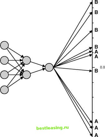

1- -1.0

Figure 7.11 Running a neural network on 10 examples from the validation set can help determine how to interpret results.

Neural Networks for Time Series

In many business problems, the data naturally falls into a time series. Examples of such series are the closing price of IBM stock, the daily value of the Swiss franc to U.S. dollar exchange rate, or a forecast of the number of customers who will be active on any given date in the future. For financial time series, someone who is able to predict the next value, or even whether the series is heading up

or down, has a tremendous advantage over other investors. Although predominant in the financial industry, time series appear in other areas, such as forecasting and process control. Financial time series, though, are the most studied since a small advantage in predictive power translates into big profits.

Neural networks are easily adapted for time-series analysis, as shown in Figure 7.12. The network is trained on the time-series data, starting at the oldest point in the data. The training then moves to the second oldest point, and the oldest point goes to the next set of units in the input layer, and so on. The network trains like a feed-forward, back propagation network trying to predict the next value in the series at each step.

Time lag

Historical units

Hidden layer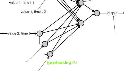

value 1, time t+1

value 2, time t-1

value 2, time t-2

Figure 7.12 A time-delay neural network remembers the previous few training examples and uses them as input into the network. The network then works like a feed-forward, back propagation network.