Self-Organizing Maps

Self-organizing maps (SOMs) are a variant of neural networks used for undirected data mining tasks such as cluster detection. The Finnish researcher Dr. Tuevo Kohonen invented self-organizing maps, which are also called Kohonen Networks. Although used originally for images and sounds, these networks can also recognize clusters in data. They are based on the same underlying units as feedforward, back propagation networks, but SOMs are quite different in two respects. They have a different topology and the back propagation method of learning is no longer applicable. They have an entirely different method for training.

What Is a Self-Organizing Map?

The self-organizing map (SOM), an example of which is shown in Figure 7.13, is a neural network that can recognize unknown patterns in the data. Like the networks weve already looked at, the basic SOM has an input layer and an output layer. Each unit in the input layer is connected to one source, just as in the networks for predictive modeling. Also, like those networks, each unit in the SOM has an independent weight associated with each incoming connection (this is actually a property of all neural networks). However, the similarity between SOMs and feed-forward, back propagation networks ends here.

The output layer consists of many units instead of just a handful. Each of the units in the output layer is connected to all of the units in the input layer. The output layer is arranged in a grid, as if the units were in the squares on a checkerboard. Even though the units are not connected to each other in this layer, the grid-like structure plays an important role in the training of the SOM, as we will see shortly.

How does an SOM recognize patterns? Imagine one of the booths at a carnival where you throw balls at a wall filled with holes. If the ball lands in one of the holes, then you have your choice of prizes. Training an SOM is like being at the booth blindfolded and initially the wall has no holes, very similar to the situation when you start looking for patterns in large amounts of data and dont know where to start. Each time you throw the ball, it dents the wall a little bit. Eventually, when enough balls land in the same vicinity, the indentation breaks through the wall, forming a hole. Now, when another ball lands at that location, it goes through the hole. You get a prize-at the carnival, this is a cheap stuffed animal, with an SOM, it is an identifiable cluster.

Figure 7.14 shows how this works for a simple SOM. When a member of the training set is presented to the network, the values flow forward through the network to the units in the output layer. The units in the output layer compete with each other, and the one with the highest value wins. The reward is to adjust the weights leading up to the winning unit to strengthen in the response to the input pattern. This is like making a little dent in the network.

The output units compete with each other for the output of the network.

The output layer is laid out like a grid. Each unit is connected to all the input units, but not to each other.

The input layer is connected to the inputs.

Figure 7.13 The self-organizing map is a special kind of neural network that can be used to detect clusters.

There is one more aspect to the training of the network. Not only are the weights for the winning unit adjusted, but the weights for units in its immediate neighborhood are also adjusted to strengthen their response to the inputs. This adjustment is controlled by a neighborliness parameter that controls the size of the neighborhood and the amount of adjustment. Initially, the neighborhood is rather large, and the adjustments are large. As the training continues, the neighborhoods and adjustments decrease in size. Neighborliness actually has several practical effects. One is that the output layer behaves more like a connected fabric, even though the units are not directly connected to each other. Clusters similar to each other should be closer together than more dissimilar clusters. More importantly, though, neighborliness allows for a group of units to represent a single cluster. Without this neighborliness, the network would tend to find as many clusters in the data as there are units in the output layer-introducing bias into the cluster detection.

The winning output unit and its path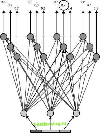

Figure 7.14 An SOM finds the output unit that does the best job of recognizing a particular input.

Typically, a SOM identifies fewer clusters than it has output units. This is inefficient when using the network to assign new records to the clusters, since the new inputs are fed through the network to unused units in the output layer. To determine which units are actually used, we apply the SOM to the validation set. The members of the validation set are fed through the network, keeping track of the winning unit in each case. Units with no hits or with very few hits are discarded. Eliminating these units increases the run-time performance of the network by reducing the number of calculations needed for new instances.

Once the final network is in place-with the output layer restricted only to the units that identify specific clusters-it can be applied to new instances. An