

|
|

|
Промышленный лизинг
Методички
Population vs Home Value Manhattan, New York Scarsdale, Westchester <0 Brooklyn, 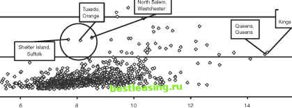 Log Population Figure 8.1 Based on 2000 census population and home value, the town of Tuxedo in Orange County has Shelter Island and North Salem as its two nearest neighbors. One possible combination function would be to average the most common rents of the two neighbors. Since only ranges are available, we use the midpoints. For Shelter Island, the midpoint of the most common range is $1,000. For North Salem, it is $1,250. Averaging the two leads to an estimate for rent in Tuxedo of $1,125. Another combination function would pick the point midway between the two median rents. This second method leads to an estimate of $977 for rents in Tuxedo. As it happens, a plurality of rents in Tuxedo are in the $1,000 to $1,500 range with the midpoint at $1,250. The median rent in Tuxedo is $907. So, averaging the medians slightly overestimates the median rent in Tuxedo and averaging the most common rents slightly underestimates the most common rent in Tuxedo. It is hard to say which is better. The moral is that there is not always an obvious best combination function. Challenges of MBR In the simple example just given, the training set consisted of all towns in New York, each described by a handful of numeric fields such as the population, median home value, and median rent. Distance was determined by placement on a scatter plot with axes scaled to appropriate ranges, and the number of neighbors arbitrarily set to two. The combination function was a simple average. All of these choices seem reasonable. In general, using MBR involves several choices: 1. Choosing an appropriate set of training records 2. Choosing the most efficient way to represent the training records 3. Choosing the distance function, the combination function, and the number of neighbors Lets look at each of these in turn. Choosing a Balanced Set of Historical Records The training set is a set of historical records. It needs to provide good coverage of the population so that the nearest neighbors of an unknown record are useful for predictive purposes. A random sample may not provide sufficient coverage for all values. Some categories are much more frequent than others and the more frequent categories dominate the random sample. For instance, fraudulent transactions are much rarer than non-fraudulent transactions, heart disease is much more common than liver cancer, news stories about the computer industry more common than about plastics, and so on. Team-Fly® To achieve balance, the training set should, if possible, contain roughly equal numbers of records representing the different categories. TIP When selecting the training set for MBR, be sure that each category has roughly the same number of records supporting it. As a general rule of thumb, several dozen records for each category are a minimum to get adequate support and hundreds or thousands of examples are not unusual. Representing the Training Data The performance of MBR in making predictions depends on how the training set is represented. The scatter plot approach illustrated in Figure 8.2 works for two or three variables and a small number of records, but it does not scale well. The simplest method for finding nearest neighbors requires finding the distance from the unknown case to each of the records in the training set and choosing the training records with the smallest distances. As the number of records grows, the time needed to find the neighbors for a new record grows quickly. This is especially true if the records are stored in a relational database. In this case, the query looks something like: SELECT distance(),rec.category FROM historical records rec ORDER BY 1 ASCENDING; The notation distance() fills in for whatever the particular distance function happens to be. In this case, all the historical records need to be sorted in order to get the handful needed for the nearest neighbors. This requires a full-table scan plus a sort-quite an expensive couple of operations. It is possible to eliminate the sort by walking through table and keeping another table of the nearest, inserting and deleting records as appropriate. Unfortunately, this approach is not readily expressible in SQL without using a procedural language. The performance of relational databases is pretty good nowadays. The challenge with scoring data for MBR is that each case being scored needs to be compared against every case in the database. Scoring a single new record does not take much time, even when there are millions of historical records. However, scoring many new records can have poor performance. Another way to make MBR more efficient is to reduce the number of records in the training set. Figure 8.2 shows a scatter plot for categorical data. This graph has a well-defined boundary between the two regions. The points above the line are all diamonds and those below the line are all circles. Although this graph has forty points in it, most of the points are redundant. That is, they are not really necessary for classification purposes. 1 2 3 4 5 6 7 8 9 10 11 12 13 14 15 16 17 18 19 20 21 22 23 24 25 26 27 28 29 30 31 32 33 34 35 36 37 38 39 40 41 42 43 44 45 46 47 48 49 50 51 52 53 54 55 56 57 58 59 60 61 62 63 64 65 66 67 68 69 70 71 72 73 74 75 76 77 78 79 80 81 82 83 84 85 86 87 88 89 90 91 92 93 94 [ 95 ] 96 97 98 99 100 101 102 103 104 105 106 107 108 109 110 111 112 113 114 115 116 117 118 119 120 121 122 123 124 125 126 127 128 129 130 131 132 133 134 135 136 137 138 139 140 141 142 143 144 145 146 147 148 149 150 151 152 153 154 155 156 157 158 159 160 161 162 163 164 165 166 167 168 169 170 171 172 173 174 175 176 177 178 179 180 181 182 183 184 185 186 187 188 189 190 191 192 193 194 195 196 197 198 199 200 201 202 203 204 205 206 207 208 209 210 211 212 213 214 215 216 217 218 219 220 221 222 |