The base values of the parameters for the numerical analysis are listed in Appendix C, Section A. The values for the moments are consistent with a sample distribution of monthly spot wheat prices taken from the Statistical Annual 1978 Chicago Board of Trade. Appendix С also shows the coefficients of the equilibrium price functions in Section B, and the coefficients of the demand functions (9) in Section C, implied by the base parameter values. Predictably, time 2 demand is a decreasing function of the contemporaneous price P2. The coefficient of P1 in the time 2 demand function is - 0.06. Thus, a decrease in Pl9 like an increase in P2, is good news in the sense of Milgrom (1981); this is confirmed by the negative dependence of \ia on P1 shown in Section D.8

To better understand this result, note that9

cov(w, Рг I уЛ9 ya, P29 So) = ft var(w уЛ9 уй9 P29 30)

- Yi cov(w, x, I уЛ9 уй9 P29 So) AVL-TiC (11)

In our example, the values of ft, yl9 ft, y29 and are positive. If the conditional covariance of и and Px were also positive, then observing a large value of Px would be good news and the investors time 2 risky asset demand would increase. In our example, however, the conditional covariance is negative given the base parameter values, so that the investor demands less of the risky asset at time 2 conditional on a high time 1 price. A high Px is viewed as bad news conditional on P2 because yC > ft VM, which implies that the investor believes a large P1 is more likely due to small supply than to favorable information about u. Hence, because y29 ft > 0, he revises downward the inferences about и initially made conditional on P2.

Now consider an uninformed, price-taking investor arriving in the market at time 2 and observing only the current price P2, the prior information So, and, possibly, the historical price, Px. This investor receives no private signal and can be considered a technician, as opposed to a fundamental investor. 10 Prices are determined by the infinite number of rational fundamental investors described in Section 1.1.

Given constant absolute risk aversion R, the maximum number of units of the riskless asset the technician will pay to observe the historical price

8 This result is similar to one of Admati (1985). She demonstrates in a single-period framework with multiple assets that a price increase may be associated with bad news.

9 Although и and xx are unconditionally uncorrelated, they are correlated conditional on P2. Provided that & and y2 are positive, the equilibrium price function (5a) implies that a high (low) и must be accompanied by a high (low) xx, holding P2 and x2 constant. The numerical results demonstrate a positive cov(m, xx\yiX,

Уа, Рг, Hi).

10 The informative value of Px is greater than it would be if the technician received private information. Nonetheless, the previous results of this section demonstrate that a rational investor who observes yn and уa is willing to pay to observe Px at time 2.

in addition to S0 and P2 (observed costlessly), is11

var(w P2, So)

7Г = log

yar(w I Pl9 P2, So).

An interpretation of the size of тг is provided by examination of the correlation of и and Px conditional on P2 and S0. The difference between the variance of и for the technician conditional on Px and that conditional on both Px and P2 can be written

Г l г> ~ Л ( I d n ~Л CQV(U, Px I P2, So)2

var(w I P2i &o) - var(w Pu P2, a0) =-(u , p w л

Equality (12) and the definition of the correlation coefficient provide

Corr(w, Px IP2i So)2 = 1 ~ ехр(-2Ятг)

Thus, 7г increases in the absolute level of the conditional correlation between и and Pv

Figures 1,2, and 4 plot it as a proportion of E( dr2P2 \ S0), the unconditional expected value of the technicians time 2 risky asset position. Because 7r and E(dT2P21S0) are proportional to risk aversion and are units of the risk-free asset, their ratio is independent of R and is unitless. For our base case, a technician would be willing to spend up to 0.127% of the value of his expected risky asset investment on ТА. If the expected risky asset investment were $100,000, for example, then the technician would be willing to spend $127 to observe historical price.

Figure 1 shows that a decrease in the variance of the historical fundamental information sx and/or the variance of the current fundamental information 52 leads to an increase in the value of ТА over most of the range of the variances examined. This relationship is reversed, however, for relatively small values of either variance.

When 5j (s2) is large relative to its base value, the fundamental investors demands place little weight on yn (yt2) because the signal is relatively uninformative. Indeed, prices become jointly nearly uninformative of и as sx and 52 approach infinity. Accordingly, the technician is unwilling to pay much for past price in these circumstances. As either sx or s2 declines, fundamental investors demands place increasing weight on private information, and 02 increases while y2 and 52 decrease. An implication of the decline in 52 is that the current and the historical prices become jointly more revealing of the asset payoff и and the historical supply increment xx. A second, opposing effect is that the current price alone becomes more revealing of the asset payoff as 02 becomes large. This implies that the observance of Px is not very useful when sx or s2 approaches zero; in the

11 See equation (3.1) of Admati and Pfleiderer (1986) and their associated discussion.

0.09-j O.OB-j 0.07-

a 0.06-t

0.05-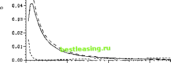

0 100 200 300 400

Variance of signal error

Figure 1

The ratio of the value of technical analysis and expected time 2 investment of the technician, ж/Е{йггР2\% shown as a function of the variance of the supply increment, V?. The solid line represents the case in which both V\ and V\ are varied, the short-dashed line the case in which only V\ is varied, and the long-dashed line the case in which only V\ is varied.

0.20-j- 0.18-j л 0.16- 1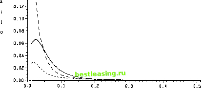

Variance of supply increment

Figure 2

The ratio of the value of technical analysis and expected time 2 investment of the technician, it/E{drlP21 Ho}, shown as a function of the variance of the noise, s in private signals, yu- The solid line represents the case in which both sx and s2 are varied, the short-dashed line the case in which only is varied, and the long-dashed line the case in which only s2 is varied.