0.6 j

0.5-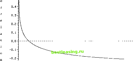

~0-3 I.........I 1 1 1 1 i 1 1 i 1 1 i i ........ 4 .......

0 100 200 300 400 500

Variance of the supply increment V\

Figure 3

The conditional correlation of и and Р1У corr(t#, Px P2, H0) as a function of V\, the variance of the time 1 per capita supply increment хг. The values of the other parameters are set equal to the base values shown in Section A of Appendix C.

limit, Px = P2 = и (P2 = u) when sx = 0 (s2 = 0). It appears from Figure 1 that at moderate to high initial levels of signal variance, the first of these two effects dominates and the value of ТА increases as sx or s2 falls. The second effect dominates for low levels of signal variance so that the value of ТА declines as the precision of the fundamental information increases.

Figure 2 shows changes in the value of ТА due to changes in the variances of the supply increments, that is, changes in noise. It is evident that changes in the value of ТА are directly related to changes in historical noise, V\, for large V\ and inversely related for very small V\. The relation for the technician analogous to Equation (11), that is,

cov(w, PX\P2, So) = ftvarCMlPz, So) - 7iCOv(w, xx\P2, S0) (Ha)

helps in understanding the relationship between V\ and the value of ТА.

For relatively large values of V\, variations in Px are primarily due to variations in xx. Hence cov(w, xx\P2, S0) is relatively large and, as shown in Figure 3, corr(w, Рг \ P29 S0) < 0. The technician finds high (low) values of Px to be bad (good) news. When V\ is small the conditional correlation of и and Px is positive because xx has little influence; high values of Px are good news. With intermediate values of V\, that is, those near V\ = 45, the value of ТА is small. For values in this range, it is difficult to discriminate between variations in Px to и and those due to xx conditional on observing P2.

Unlike variations in V\, variations in V\ and V\ = V\ from the base values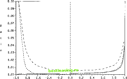

Correlation of the supply increments p

Figure 4

The ratio of the value of technical analysis and expected time 2 investment of the technician, v/EQdnPz IH0), shown as a function of p, the correlation of the supply increments хг and x2. The

solid line represents the case in which V\= V\ = 226, the short-dashed line the case in which V\ = 113 and V\ = 226, and the long-dashed line the case in which V\ = 226 and V\ = 113. The values of the remaining parameters are set equal to the base values shown in Section A of Appendix С

provide no cases in which corr(w, Px \ P2l S0) = 0. As documented by Figure 2, a rise in the current noise, V\, decreases the value of ТА, independently of the initial value of V\. When V\ is small, neither the current nor the historical price is perturbed significantly by x2 so the prices jointly reveal the asset payoff and the time 1 supply increment xx with great accuracy. ТА has considerable value. This is to be contrasted with the limiting case V\ = 0 in which the current price alone reveals the payoff and ТА has no value. When the noisy variation in P2 due to x2 is large, there is little to gain from observing Px because the technical analyst still must infer three unknowns from only two prices. Furthermore, because the risk-averse investors time 1 demands, (6b), are inversely related to the variance of P2, the sensitivity of Px to changes in private information is reduced as V\ rises. In the limit, as V\ goes to infinity, it is impossible to learn anything about и from Px becaiise the investors refuse to act on their private information at time 1.

Note that as V\ = V\ declines from relatively low levels, the value of ТА declines. This is to be contrasted with the increase in the value of ТА as either V\ or V\ declines individually. One finds that the current price is highly correlated with both the asset payoff and the historical price when both the current and historical noises are small. Hence there is little left to learn from the historical price once the current price is observed. In

the limit, as V\ and V\ jointly approach zero, P2 alone reveals u, and Px is worthless to the technician.

Figure 4 illustrates variations in the value of ТА as p is altered. For extreme values of the correlation between the supply shocks, p = 1, per capita supplies are identified by a single variable, that is, x2 = qxx for some constant q, and current price is perfectly revealing; ТА has no value. Nonetheless, provided that xx + x2 does not approach zero, the value of ТА increases as p approaches 1. This follows from the fact that the three unknowns u, xXl and x2 are revealed with great accuracy by the joint use of current and historical price. One sees from Figure 4 that the value of ТА does increase as p approaches 1 when V\ Ф V\ and as p approaches 1 when V\ = V\. In the case V\ = V\, the time 2 per capita supply goes to zero (almost surely) as p approaches - 1 and P2 becomes nearly perfectly revealing of и leaving little to be learned from the historical price.

Historical attempts to judge the value of ТА generally were based on examinations of the unconditional moments of asset returns or price changes. We have shown that, in this model, the value of ТА is zero if and only if the conditional covariance cov( и, Px \ P2, S0) is zero. It is of interest, therefore, to examine the relation between this covariance and the unconditional moments of the price changes. The definition of covariance and the law of iterated expectations allows one to write the unconditional covariance of price changes as

cov(w - P2, P2 - Px I Ho) = £[cov(w - P2, P2 - Px I P2, Ho) I So]

+ cov[£(w- P2 I Pn So),

E{P2 - Px I P2, So) I So]

= A + В

The normality of the random variables implies A = -cov(u, РХ\РЪ S0). Hence, one may examine the unconditional covariance of price changes to determine whether ТА has value only if the covariance of conditional expected price changes, Д is known.

Figure 5 displays the value of corr(w - P2l P2 - ЛН0) as a function of the correlation between per capita supply increments, p, and it is to be compared to Figure 4. One finds that, in this equilibrium, В Ф 0, a fact shown by the difference between (1) the value of p at the zero level of the short-dashed line in Figure 5 (p = -0.16) and (2) the analogous p in Figure 4 (p = -0.42). Furthermore, В varies with p and the other exogenous parameters. This suggests that empirical studies of the value of ТА should not rely on the assumption that conditional expected price changes are uncorrelated.

3. Is the Equilibrium Weak-Form Efficient?

The fact that technical analysis has value in this market setting raises the question, Is the market, that is, the noisy rational expectations equilib-