lios. Ratios of the cross-autocovariances may be formed to estimate relative nontrading proba&Mities for portfolios, since

Covf;, r;;l+ ]

(3.1.29)

In addition, for purposes of testing the overall specification of the non-trading model, these ratios give rise to many over-identifying restrictions, since

yw,(n) yK,K,(n) YwM) Уч. ,*,( ) Y* У*, (п) Kr,r,( ) Y*,*№) )W, ( ) Yt,

tin) = /яЛ

r,( ) \Л )

(3.1.30)

for (any arbitrary sequence of distinct indices K\,к-г,...л к а ф lh г < Д/; where Щ is the number of distinct portfolios and п-Л)(п) = Cov] >;(+11]. Thejrefore, although there are distinct autocovarianccs in Г , the restrictions implied by the nontrading process yield far fewer degrees of freedom.

Tinw Aggregation

The discrete-time framework we have adopted so far docs not require the specjfication of the calendar length of a period. This advantage is more apparent than real since any empirical implementation of the nontrading model (3.1.2)-(3.1.3) must cither implicitly or explicitly define a period to be a particular fixed calendar time interval. Once the calendar time interval has been chosen, the stochastic behavior of coarser-sampled data is restricted by the parameters of the most finely sampled process. For example, if the length of a period is taken to be one day, then the moments of observed monthly returns may be expressed as functions of the parameters of the daily observed returns process. We derive such restrictions in this section.

To do this, denote by r? (q) the observed return of security i at lime r where one unit of r-time is equivalent to q units of Mime, thus:

(3.1.31)

Then under the nontrading process (3.1.2)-(3.1.3), it can be shown that Ж the time-aggregated observed returns processes r, (7)} (г = 1...../V) are

covariance-stationary with the following first and second moments (see l.o Ж and MacKinjay 11990a]):

V-Klq)] = qti, Var[ r;t(<7)] = qe; +

2тг,(1 - я,7) (1 - я,)-

(3.1.32) (3.1.33)

I - я/4 2

1 - я,

ф j, n > 0. (3.1.3b)

where s ц,/о, as before.

Although expected returns lime-aggregate linearly, (3.1.33) shows (hat variances do not. As a result of the negative serial correlation in r the variance of a sum is less than the sum of the variances. Time aggregation does not affect the sign of the autocorrelations in (3.1.35) although their magnitudes do decline with the aggregation value q. As in (3.1.12), die autocorrelation of time-aggregated returns is a nonposilive continuous function of я, on (0, 1) which is /.его at я, = 0 and approaches /его as Я; approaches unity, and hence it attains a minimum.

To explore the behavior of the fust-order autocorrelation, we plot it as a function of я, in Figure 3.1 for a variety of values of q and £: q takes on the values 5, 22, (Hi, and 244 to correspond lo weekly, monthly, quarterly, and annual returns, respectively, since q = 1 is taken to be one day, and 5 takes on the values 0.09, 0.10, and 0.21 to correspond to daily, weekly, and monthly returns, respectively. Figure 3.1 a plots the fust-order autocorrelation p\((>) for the four values of с/ with £ = 0.09. The curve marked V/ = 5 shows that the weekly first-order autocorrelation induced by nouirading never exceeds -5% and only attains that value with a daily nontrading probability in excess of 90%.

Although the autocorrelation of coarser-sampled returns such as monthly or quarterly have more extreme minima, they are attained only at higher nontrading probabilities. Also, time-aggregation need not always yield a more negative autocorrelation, as is apparent from the portion ol the graphs to the left of, say, л = .80; in that region, an increase in the aggregation value </ leads lo an autocorrelation closer to /его. Indeed as 17 increases without bound the autocorrelation (3.1.35) approaches zero for fixed я аи(1 thus nontrading has little impact on longer-horizon returns.

Values lor £ were obtained by taking ibe ratio ol ilie sample mean to the sample .standard deviation for daily, weekly, and monthly equal-weighted slock returns indexes (or the sample period from IMiV! lo 1987 as reported in l.o and MacKinlay (I.IHK, fables la-r). Although these values may be more representative of slock indexes radiei (ban individual securities, nevertheless for I lie sake ol illustration they should sullii e.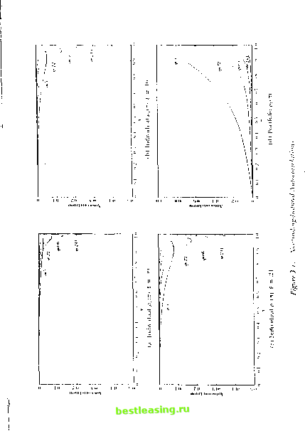

The effects of increasing £ are traced out in Figures 3.1b and 3.1c. Even if we assume £ = 0.21 for daily data, a most extreme value, the nontrading-induced autocorrelation in weekly returns is at most -8% and requires a daily nontrading probability of over 90%. From (3.1.8) we see that when я, - .90 the average duration of nontrading is nine days! Since no security listed on the New York or American Stock Exchanges is inactive for two weeks (unless it has been delisted), we infer from Figure 3.1 that the impact of nontrading for individual short-horizon stock returns is negligible.

Time Aggregation For Portfolios

Similar time-aggregated analytical results can be derived for observed portfolio returns. Denote by r°r(q) the observed return of portfolio A at time r where one unit of т-time is equivalent to q units of Mime; thus

(3.1.37)

i=(t-D?+i

where r°al is given by (3.1.19). Then under (3.1.2)-(3.1.3) the observed portfolio returns processes \r°r(q)} and [r£t(q)} are covariance-stationary with the following first and second moments as Na and N4 increase without bound:

Var[r;t(?)] =5= Согг[£(,).£+11(,)] A

Cov[C(r/),r;t+ (?)]

<7-2тг.

1 - лу 1 +**

х лу fix aj, и > 0

<7(1-)-2яЛ1-я,)

1-яЛ2

(3.1 (3.1

(3.1

п > 0 (3.1

.38) .39)

40) 41)

П-я.Ю-л ) п2

for n = 0

.ТЙ] *r*lfi.b°f for n>0

(3.1.42)

for к = a, b, q > 1, and arbitrary portfolios a, 6, and time r.

Equation (3.1.40) shows thai time aggregation also affects ihe autocorrelation of observed portfolio returns in a highly nonlinear fashion. In contrast to the autocorrelation for time-aggregated individual securities, (3.1.40) approaches unity for any fixed q as nK approaches unity; therefore the maximal autocorrelation is one.

To investigate the behavior of the portfolio autocorrelation we plot it as a function of the portfolio nontrading probability л in Figure 3.1d for q = 5, 22, 66, and 244. Besides differing in sign, portfolio and individual autocorrelations also differ in absolute magnitude, the former being much larger than the hitler for a given nontrading probability. If the non-trading phenomenon is extant, it will he most evident in portfolio returns. Also, portfolio autocorrelations are monotonically decreasing in q so that lime aggregation always decreases nontrading-induced serial dependence in portfolio returns. This implies that we are most likely lo find evidence of nontrading in short-horizon returns. Wc exploit both these implications in the empirical analysis of Section 3.4.1.

3.1.2 Extensions and Generalizations

Despite the simplicity of the model of nonsynchronous trading in Section 3.1.1, its implications for observed time series are surprisingly rich. The framework can be extended and generalized in many directions with little difficulty.

It is a simple matter to relax the assumption thai individual virtual re-turntOarc IID by allowing the common factor to be autocorrelaled and the distu bances to be cross-scclionally correlated. For example, allowing J, to be a stationary AR(1) is conceptually straightforward, although the calculations become somewhat more involved. This specification will yield a decomposition of observed autocorrelations into two components: one due to the common factor and another due to nontrading.

Allowing cross-sectional dependence in the disturbances also complicates the moment calculations but does not create any intractabilities.lr Indecjd, generalizations to multiple factors, time-series dependence of the disturbances, and correlation between factors and disturbances are only limited W ihe patience and perseverance of the reader; the necessary moment calumnious are not intractable, but merely tedious.

Dependence can be built into the nontrading process itself by assuming that llje5 s are Markov chains, so that the conditional probability of trading

1 Asjwe discussed earlier, some lor m ol t ross-scctioual weak dependence must be imposed so that jibe asymptotic arguments of the portfolio results still obtain. Of course, such an a4sunipion may mil always be appropriate as. for example, in the case ol companies within the same inclustn. whose residual risks wc might expect to be positively correlated. 1 hereloie. the asymptotic approximation will be most accurate tor vscll-divci silted portfolios.

tomorrow depends on whether or not a trade occurs today. Although this specification does admit compact and elegant expressions for the moments ol the observed returns process, we shall leave their derivation to the reader (see Problem 3.3). However, a brief summary of the implications for the lime-series properties of observed returns may be worthwhile: (1) Individual security returns may be positively autocorrelaled and portfolio returns may be negatively autocorrelaled, but these possibilities arc unlikely given empirically relevant parameter values; (2) It is possible, but unlikely, for autocorrelation matrices to be symmetric; and (3) Spurious index autocorrelation induced by nontrading is higher (or lower) when there is positive (or negative) persistence in uoulradiug. In principle, property (3) might be sufficient to explain die magnitude of index autocorrelations in recent stock market dala. However, several calibration experiments indicate the degree of persistence in nontrading required to yield weekly autocorrelations of 30% is empirically implausible (see l.o and MacKinlay [1990c] for details).

One final direction for further investigation is the possibility of dependence between the nontrading and virtual returns processes. If virtual re-turns arc taken lo be new information then the extent to which traders exploit this information in determining when (and what) to trade will show itself as correlation between Гц and <$ . Many strategic considerations are involved in models of information-based trading, and an empirical analysis of such issues promises Lo be as challenging as il is exciting.

However, if it is indeed the case that return autocorrelation is induced by information-based nontrading, in what sense is this autocorrelation spurious? The premise of the extensive literature on nonsynchroiious trading is that nontrading is an outcome of institutional features such as lagged adjustments and nonsynchronously reported prices. But il nonsynchronicily is purposeful and infonnalionally motivated, (hen the serial dependence it induces in asset returns should be considered genuine, since il is the result of economic forces rather than measurement error. In such cases, purely statistical models of nontrading are clearly inappropriate and an economic model of strategic interactions is needed.

3.2 The Bid-Ask Spread

One of the most important characteristics that investors look for in an organized financial market is liquidity, the ability to buy or sell significant

Some good illustrations of the kind ot Hading behaviot that tan arise Iroili strategic considerations are contained in Admati and Illeidcrer (I.IHH. IWI). bcnsimas and I л (ИИМ>), Kaslcv and Ollara (l< 87, I WO). Kyle (I.W.i), and Wang (lilr.t. I.IM).