

|
|

|
Промышленный лизинг
Методички
j. niamei micmsliuclure - jj, + and so on. For simplicity, the state-space partition of S is usually defined lo he intervals: /1, = (-00, ffi] (3.3.1(5) /,. . s ( , . a2] (3.3.17) Л, = < , or,-] (3.3.18) Л, = (<*, , , oo). (3.3.19) Althnugl 1 the observed price change can be any number of ticks, positive or negative, we assume that 111 in (3.3.15) is finite lo keep the number of unknown parameters Finite. This poses no difficulties since we may always let some stales in <S represent a multiple (and possibly countably infinite) number of values for the observed price change. For example, in the empirical application of I lausman, l.o, and MacKinlay (1992), s\ is defined to be a price change of-I ticks or less, V to be a price change of+4 ticks or more, and *> to .% lo be price changes of -3 licks to +3 ticks, respectively. This parsimony is obtained at die cost of losing price resolution. That is, under this specification the ordered probit model does not distinguish between price changes of +4 and price changes greater than +4, since the -f-4-lick outcome and the greater than +4-tick outcome have been grouped together into a common event. The same is true for price changes of -4 licks and price changes less than -4. This partitioning is illustrated in Figure 3.4 which superimposes the partition boundaries (a,) on the density function of 1 , and the sizes of the regions enclosed by the partitions determine the probabilities n, of the discrete events. Moreover, in principle the resolution may be made arbitrarily finer by simply introducing more slates, i.e., by increasing m. As long as (3.3.14) is correctly specified, increasing price resolution will not affect the estimated /? asymptotically (although finite-sample properties may differ). However, in practice the data will impose a limit on (he fineness of price resolution simply because there will be no observations in the extreme states when in is too large, in which case a subset of the parameters is not identified and cannot be estimated. The Conditional Distribution ol Trice Changes Observe that the f/js in (3.3.14) are assumed to be nnnidcntieally distributed, conditioned on the Xis. The need for this somewhat nonstandard assumption comes from (he irregular and random spacing of transactions data. If, for example, transaction prices were determined by the mode! in Marsh and Rosenfeld (1980) where the Is are increments of arithmetic J.J. ModelingTransactions Data 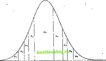 Figure 3.4. The Ordered Probit Model Brownian motion with variance proportional to Д/* = /* - tk-\, <7A2 must be a linear function of Atk which varies from one transaction to the next. I More generally, to allow for more general forms of conditional jhel-eroskedasticity, let us assume that al is a linear function of a vector of predetermined variables W* = [ Wu WLk ] so that E[ X*.W ] = 0, ekWlDU<fl,af) (3.3.20) al = Y5 + Y?Wlk + --- + ylWu (3.3.21) where (3.3.20) replaces the corresponding hypothesis in (3.3.14) and the conditional volatility coefficients \yj) are squared in (3.3.21) to ensure fpt the conditional volatility is nonnegative. In this more general framework, the arithmetic Brownian motion model of Marsh and Rosenfeld (1986) tpan be easily accommodated by setting j Xk[3 = nAtk (3.3.22) al = у2Д(*. (3.3.23) In this case, Vfk contains only one variable, Atk (which is also the only variable contained in Xk). The fact that the same variable is included in both X; and W* does not create perfect multicollinearity since one vector affects the conditional mean of Yk while the other affects the conditional variance. 3£ Ж The dependence structure of the observed process Yk is clearly induced by that of Yk and the definitions of the A/s, since P( П = sj i = л,) = p( y; e л, i y; , б Л, ). (3.3.24) As a consequence, if X and Wi. arc temporally independent, die observed process Yk is also temporally independent. Of course, these arc fairly restrictive assumptions and are certainly not necessary for any of the statistical inferences that follow. We require only that the e*s be conditionally independent, so that all serial dependence is captured by the X),s and the W/,s. Consequently, the independence of the e/s does not imply that the Yt a are independently distributed because no restrictions have been placed on the temporal dependence of the Xj,s or Wis. 0 The conditional distribution of observed price changes Yk, conditioned on X and W>, is determined by the partition boundaries and the particular distribution of e*. For normal eVs, the conditional distribution is POi = i.fXbW.) j = Р(Хк(3 + ек e A, I X*.W ) j P(X;/3 4-c < a, I XA,W*) j = P(a, , < Хк(3 + {к < a, I XA,W*) j 1р(оги-1 < Хк0 + ек I XA,W* ) i= 1 (3.3.25) (3.3.20) if / = 1 if 1 < i < m i - in. (3.3.27) where CT (Wn) is written as an argument ofW* to show how the conditioning variables enter the conditional distribution, and Ф(-) is the standard normal cumulative distribution function. To develop some intuition for the ordered probit model, observe that the probability of any particular observed price change is determined by where the conditional mean lies relative to the partition boundaries. Therefore, for a given conditional mean X\(3, shifting the boundaries will alter the probabilities of observing each state (see Figure 3.4). ln fact, by shifting the boundaries appropriately, ordered probit can lit any arbitrary multinomial distribution. This implies that the assumption of normality underlying ordered probit plays no special role in determining the probabilities of states; a logistic distribution, for example, could have served equally well. However, since it is considerably more difficult to capture conditional heteroskedasticity in the ordered logit model, we have chosen the normal distribution. Given the partition boundaries, a higher conditional mean X\fi implies a higher probability of observing a more extreme positive stale. Of course, the labeling of states is arbitrary, but the ordered probit model makes use of the natural ordering of die states. The regressors allow us to separate the effects of various economic factors that influence the likelihood оГопс state versus another. For example, suppose that a large positive value of X usually implies a large negative observed price change and vice versa. Then the ordered probit coefficient fi\ will be negative in sign and large in magnitude (relative to a*, of course). Ry allowing the data to determine the partition boundaries a, the coefficients /3 of the conditional mean, and the conditional variance стк, the ordered probit model captures the empirical relation between the unol>-servable continuous state space S and the observed discrete state space S as a function of the economic variables X* and W . Maximum Likelihood Estimation Let Ik(i) be an indicator variable which lakes on the value one if the realization of the /ith observation Yk is the ith slate s and zero otherwise. Then the log-likelihood function С for die vector of price changes Y = I )i Y-2 Y }, conditional on the explanatory variables X = I X, X-> X ] and W = [W, W2 W ], is given by £(Y,X.W) = Ejlogo(i) L V cr*lW.) J \ <7.(WA) + /,w,),og[.-o(il)]J. (з 28) Although <7д- is allowed to vary linearly with WA, there are some constraints that must be placed on the parameters lo achieve identification since, lor example, doubling the as, the /3s, and ok leaves the likelihood unchanged. A typical identification assumption is to set j/H = I. We are then left with three issues that must be resolved before estimation is possible: (i) the number ol slates m; (ii) the specification of the regressors X ; and (iii) the specification of the conditional variance crk. In choosing hi, wc must balance price resolution against the practical constraint thai too large an m will yield no observations in the extreme slates si and s, . For example, ifwc set m to 101 and define the stales s\ and sun symmetrically lo lie price changes of -50 licks and +50 licks, respectively, we would find no )\\ among typical NYSK stock transactions falling into either ol these states, and it would he impossible to estimate the parameters associated with these two states. Perhaps the easiest method for determining hi is to use the empirical frequency distribution of the dalaset as a guide, selling m as large as possible, but not so large that the extreme stales have no observations in them.M The remaining two issues must be resolved on a casc-by-case basis since the specification for the regressors and акг are dictated largely by the particular application at hand. For forecasting purposes, laggetl price changes and market indexes may be appropriate regressors, but for estimating a structural model of marketmaker monopoly power, other variables might be more appropriate. 3.4 Recent Empirical Findings The empirical market microsituclure literature is an extensive one, straddling both academic and industry publications, and it is difficult if not impossible lo provide even a superficial review in a few pages. Instead, we shall present three specific market microstructure applications in this sec-lion, each in some depth, to give readers a more concrete illustration of empirical research in this exciling and rapidly growing literature. Section 3.4.1 provides an empirical analysis of uonsynchronous trading in which the magnitude of the nontrading bias is measured using daily, weekly, and monthly stock returns. Section 3.4.2 reviews the empirical analysis of effective bid-ask spreads based on the model in Roll (1984). And Section 3.4.3 presents an application ol the ordered probit model to transactions data. ?.-/. / Nonsynchronous 1 railing Before considering the empirical evidence for nontrading effects we summarize the qualitative implications of the nontrading model ol Section 3.1.1. Although many of these implications are consistent with other models of uonsynchronous trading, the sharp comparative static results and exposi- lKl;or example, llatisinan, l.o. anil MacKinlay (ltl.)2) scl m = 11 for the larger Mocks, implying cxlleinc stales ol - I licks or less and -И licks or more, and scl nt - Г> lor die smaller slocks, iniilviiig esurtiir stales ol 2 ticks or less and +J licks or more. Note dial although the delinilioii ol slates need not he sMiimelrii 1st.He V ran he - Ii licks ot less, iinplving thai state л., is -tlicks or more), tlx* symmetry ol the histogram of price changes in their dalaset suggests a svinmeli ic deliuiliou ot die i,s. tional simplicity are unique to this framework. Under the assumptions of Section 3.1.1, the presence of nonsynchronous trading 1. does not affect the mean of either observed individual or portfolio returns. 2. increases the variance of observed individual security returns that have nonzero means. The smaller the mean, the smaller the increase in the variance of observed returns. 3. decreases the variance of observed portfolio returns when portfolios are well-diversified and consist of securities with common nontrading probability. 4. induces geometrically declining negative serial correlation in observed individual-security returns that have nonzero means. The smaller the absolute value of the mean, the closer is the autocorrelation to zero. 5. induces geometrically declining positive serial correlation in observed portfolio returns when portfolios are well-diversified and consist of securities with a common nontrading probability, yielding an AR(1) for the observed returns process. (i. induces geometrically declining cross-autocorrelation between observed returns of securities i and j which is of the same sign as PiPj. This cross-autocorrelation is generally asymmetric: The covariance of current observed returns to i with future observed returns to j need not be the same as the covariance of current observed returns to j with future observed returns to i. The asymmetry arises from the fact that different securities may have different nontrading probabilities. 7. induces geometrically declining positive cross-autocorrelation between observed returns of portfolios A and В when portfolios are well-diversified and consist of securities with common nontrading probabilities. This cross-autocorrelation is also asymmetric and arises from the facjt that securities in different portfolios may have different nontrading probabilities. 1 8. induces positive serial dependence in an equal-weighted index if the betas of the securities are generally of the same sign, and if individual returns have small means. 9. and time aggregation increases the maximal nontrading-induced negative autocorrelation in observed individual security returns, but this maximal negative autocorrelation is attained at nontrading probabilities increasingly closer to unity as the degree of aggregation increases. 10. and time aggregation decreases the nontrading-induced autocorrelation in observed portfolio returns for all nontrading probabilities. Since the effects of nonsynchronous trading arc more apparent in se-! curilies grouped by nontrading probabilities than in individual stocks, our empirical application uses the returns of ten size-sorted portfolios for daily, 1 2 3 4 5 6 7 8 9 10 11 12 13 14 15 16 17 18 19 20 21 [ 22 ] 23 24 25 26 27 28 29 30 31 32 33 34 35 36 37 38 39 40 41 42 43 44 45 46 47 48 49 50 51 52 53 54 55 56 57 58 59 60 61 62 63 64 65 66 67 68 69 70 71 72 73 74 75 76 77 78 79 80 81 82 83 84 85 86 87 88 89 90 91 92 93 94 95 96 97 98 99 100 101 102 103 |