

|
|

|
Промышленный лизинг
Методички
/. I:venl-StudyAnalysis issue and (iud dial the analytical computations and the empirical power are very <lose. Il is difficult io rcai Ii general conclusions concerning the the ahililv ol event-study methodology to dctcel nonzero abnormal returns. When conducting an event study il is necessary to evaluate the power given the parameters and objectives ol the study. If the power seems sufficient then one ran proceed, otherwise one should search for ways of increasing the power. This can be done by increasing the sample size, shortening the event window, or by developing more specific predictions of the null hypothesis. 4.7 Nonparametric Tests The mclhodsdisi ussed lo lliispoini arc parametric in nature, in that specific assumptions have been made about the distribution of abnormal returns. Alternative nonparametric approaches are available which are free of specific assumptions concerning the distribution of returns. In this section we discuss two common nonparametric lesls for event studies, ihe sign lest and the rank test. Ihe sign test, which is based on the sign of the abnormal return, requires that the abnormal returns (or more generally cumulative abnormal returns) are independent across securities and thai the expected proportion of positive abnormal returns under the null hypothesis is 0.5. The basis ol the lest is that under ihe null hypothesis it is equally probable thai the CAR will be positive or negative. If, lor example, the alternative hypothesis is that there is a positive abnormal return associated with a given event, the null hypothesis is 11 : /; < 0.5 and the alternative is I\y. j> > 0.5 where = !V(GAR, > 0.0). To calculate the test statistic we need the number of cases where the abnormal return is positive, Ny, and the total number of cases, N. Letting /t be the test statistic, then asymptotically as N increases we have [N> I Ntr- For a lest ol size (I - ( ), 1 ln is rejected if / > Ф (а). A weakness of the sign test is that it may not be well specified if the distribution of abnormal returns is skewed, as can be the case with dailv data. With skewed abnormal returns, the expected proportion of positive abnormal returns can differ from one half even under the null hypothesis. In response to ibis possible shorn oiniiig, Corrado (1989) proposes a non-parainctric rank text for abnormal performance in event studies. We briellv describe his tesi of the null hypothesis that there is no abnormal return on 4.8. Cross-Sectional Models event day zero. The framework can be easily altered for events occurring over multiple days. Drawing on notation previously introduced, consider a sample of hi abnormal returns for each of N securities. To implement the rank test it is necessary for each security to rank the abnormal returns from 1 to Ц. Define K,T as the rank of the abnormal return of security i for event lime period r. Recall that r ranges from Tt + 1 to T-i and т = 0 is the event day. The rank test uses the fact that the expected rank under the null hypothesis event day zero is: is The test statistic for the null hypothesis of no abnormal return on Tests of the null hypothesis can be implemented using the result tha the asymptotic null distribution of /4 is standard normal. Corrado (1989) pves further details. Typically, these nonparametric tests are not used in isolation bijt in conjunction with their parametric counterparts. The nonparametric tests enable one to check the robustness of conclusions based on parametric tests. Such a check can be worthwhile as illustrated by the work of Camplbell and Wasley (1993). They find that for daily returns on NASDAQ sticks the nonparametric rank test provides more reliable inferences than dojthe standard parametric tests. j 4.8 Cross-Sectional Models Theoretical models often suggest that there should be an associationkbe-tween the magnitude of abnormal returns and characteristics specific to the event observation. To investigate this association, an appropriate tool is a cross-sectional regression of abnormal returns on the characteristics of interest. To set up the model, define у as an (Wx 1) vector of cumulative abnormal return observations and X as an (NxK) matrix of characteristics. The first column of X is a vector of ones and each of the remaining (К - 1) columns is a vector consisting of the characteristic for each event observation. Then, for the model, we have the regression equation у = X0 + r;, (4.8.1) where в is the (Kxl) coefficient vector and tj is the (Nxl) disturbance vector. Assuming Я[Хт?] = 0, we can consistently estimate в using OI.S. For the OLS estimator wc have 0 = (ХХГХу. (4.8.2) Assuming the elements of л are cross-scctionally uncorrelated and hoino-skedasde, inferences can be derived using the usual OLS standard errors. Defining oi as the variance of the elements of 77 we have Var[0] = (ХХГЦ. Using the unbiased estimator for a, (4.8.3) (N - K) (4.8.4) where r) = у - X6\ we can construct (-statistics to assess the statistical significance of the elements of в. Alternatively, without assuming homoskedaslic-ity, wc can construct hetcroskcdasticity-consislcnt z-statistics using Var[0] = -(ХХГ1 N (Xxy (4.8.5) whejre x, is the ith row ofX and f/, is the ith clement off). This expression for jhe standard errors can be derived using the Generalized Method of Moments framework in Section Л.2 of the Appendix and also follows from the rest Its of While (1980). The use of hctcroskedasticity-consislenl standard crrcrs is advised since there is no reason to expect the residuals of (4.8.1) to b: homoskedastic. Asquilh and Mullins (1986) provide an example of this approach. The two-lay cumulative abnormal return for the announcement of an equity olTc ing is regressed on the size of the offering as a percentage of the value of the total equity of the firm and on the cumulative abnormal return in the ;leven months prior to the announcement month. They find that the magnitude of the (negative) abnormal return associated with the announcement of equity offerings is related to both these variables. I-argcr pre-event cumulative abnormal returns arc associated with less negative abnormal retufns, and larger offerings arc associated with more negative abnormal returns. These findings are consistent with theoretical predictions which they discuss. One must be careful in interpreting the results of the cross-sectional regression approach. In many situations, the event-window abnormal return will be related to firm characteristics not only through the valuation effects of the event but also through a relation between the firm characteristics and the extent lo which the event is anticipated. This can happen when investors rationally use firm characteristics to forecast the likelihood of the event occurring. In these cases, л linear relation between the linn characteristics and the valuation effect of the event can be hidden. Malalesta and Thompson (1985) and Latum and Thompson (1988) provide examples of this situation. Technically, the relation between the firm characteristics and the degree of anticipation of the event introduces a selection bias. The assumption that the regression residual is uncorrelated with the regressors, K[X j] = 0, breaks down and the OLS estimators are inconsistent. Consistent estimators can be derived by explicitly allowing for the selection bias. Acharya (1988, 1993) and F.ckbo, Maksimovic, and Williams (1990) provide examples of this. Prabhala (1995) provides a good discussion of this problem and die possible solutions. He argues that, despite niisspecilication, under weak conditions, the OLS approach can be used for inferences and the (-statistics can be interpreted as lower bounds on the (rue significance level of the estimates. 4.9 Further Issues A number of further issues often arise when conducting an event study. We discuss some of these in this section. 4.9.1 Role of the Sampling Internal If the timing of an event is known precisely, then the ability to statistically identify the effect of the event will be higher for a shot let sampling interval. The increase results from reducing the variance of the abnormal return without changing the mean. We evaluate the empirical importance of this issue by comparing the analytical formula for the power of the test statistic J\ with a daily sampling interval to the power with a weekly and a monthly interval. We assume that a week consists of five days and a month is 22 days. The variance of the abnormal return for an individual event observation is assumed to be (4%)2 on a daily basis and linear in time. In Figure 4.4, wc plol the power of the test of no event-effect against the alternative of an abnormal return of 1% for 1 to 200 securities. As one would expect given the analysis of Section 4.6, the decrease in power going from a daily interval lo a monthly interval is severe. For example, with 50 securities the power for a 5% test using daily data is 0.94, whereas the power using weekly and monthly data is only 0.35 and 0.12, respectively. The clear message is that there is a substantial payoff in let 111s of increased power from reducing the length of the event window. Morse (1984) presents detailed analysis of the choice of daily versus monthly data and draws the same conclusion. 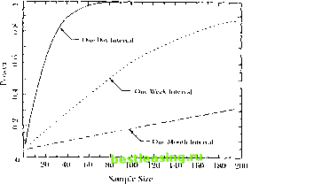 Figure 4.4. Power of Fveiit-Slmh list Statistic /, tit Reject the Nail Hypothesis that the Abnormal Return is /его. for Different Sampling Internals, Шеи Ihe Square Root of the Average Variance oj Ihe Abnormal Return Across Firms Is 4% for Ihe Daily Interval A sampling interval of otic dav is not the shoricst interval possible. Willi die increased availability ol transaction data, recent studies have used observation intervals of duration shorter than one day. The use of intra-tiaily data involves some complications, however, of the sort discmscd in Chapter 3, and so the net benefit of very short intervals is unclear. Barclay and I.il/cnberger (19ЯК) discuss die use of intra-daily data in event studies. 4.9.2 Inferences with Ivent-Date Uncertainty Thus far we have assumed that the event dale can be identified with certainly. However, in some studies it may be difficult to identify the exact date. Л common example is when collecting event dates from financial publications such as the Wall Street Journal. When the event announcement appears in the newspaper one can not be certain if the market was informed before ihe close of the market die prior trading day. If ibis is the case then the prior day is the event day; if not, then the current day is the event day. The usual method of handling ibis problem is to expand the event window to two days-dav 0 and day 4-1. While there is a cost lo expanding the event window, the results in Section l.li indicate that the power properties of two-day event windows are still good, suggesting that it is-worth bearing the cost lo avoid the risk of missing the event. Ball and Torous (1988) investigate this issue. They develop a maximum-likelihood estimation procedure which accommodates event-date uncertainty and examine results of their explicit procedure versus the informal procedure of expanding the event window. The results indicate that the informal procedure works well and there is little to gain from the more elaborate estimation framework. 4.9.3 Possible Biases Event studies are subject to a number of possible biases. Nonsynchronous trading can introduce a bias. The nontrading or nonsynchronous trading effect arises when prices are taken to be recorded at time intervals of one length when in fact they are recorded at time intervals of other possibly irregular lengths. For example, the daily prices of securities usually employed in event studies are generally closing prices, prices at which the last transaction in each of those securities occurred during the trading day. These closing prices generally do not occur at the same time each day, but by calling them daily prices, we have implicitly and incorrecdy assumed that they are equally spaced at 24-hour intervals. As we showed in Section 3.1 of Chapter 3, this nontrading effect induces biases in the moments and co-momentsof returns. The influence of the nontrading effect on the variances and covariances of individual stocks and portfolios naturally feeds into a bias for the market-model beta. Scholes and Williams (1977) present a consistent estimator of beta in the presence of nontrading based on the assumption that the true return process is uncorrelated through time. They also present some empirical evidence showing the nontrading-adjusted beta estimates of thinly traded securities to be approximately 10 to 20% larger than the unadjusted estimates. However, for actively traded securities, the adjustments are generally small and unimportant. Jain (1986) considers the influence of thin trading on the distribution of the abnormal returns from the market model with the beta estimated using the Scholes-Williams approach. He compares the distribution oflthese abnormal returns to the distribution of the abnormal returns using theiusual OLS betas and finds (hat the differences are minimal. This suggests that in general the adjustment for thin trading is not important. The statistical analysis of Sections 4.3, 4.4, and 4.5 is based on the assumption that returns are jointly normal and temporally IID. Departures from this assumption can lead to biases. The normality assumption is important for the exact finite-sample results. Without assuming normally, all results would be asymptotic. However, this is generally not a problem for event studies since the test statistics converge to their asymptotic distributions rather quickly. Brown and Warner (1985) discuss this issue. 1 2 3 4 5 6 7 8 9 10 11 12 13 14 15 16 17 18 19 20 21 22 23 24 25 26 27 28 29 [ 30 ] 31 32 33 34 35 36 37 38 39 40 41 42 43 44 45 46 47 48 49 50 51 52 53 54 55 56 57 58 59 60 61 62 63 64 65 66 67 68 69 70 71 72 73 74 75 76 77 78 79 80 81 82 83 84 85 86 87 88 89 90 91 92 93 94 95 96 97 98 99 100 101 102 103 |