

|
|

|
Промышленный лизинг
Методички
?. / he Capital Asset Pricing Model where / denotes ihe asset and / denotes the lime period, / = 1.....7 . /. and / are die reali/.ed excess returns in time period / for asset i and the market portfolio, respectively. Typically the Standard and Poors 500 Index selves as a proxy for the market portfolio, and the US Treasury hill rate proxies for the riskfree return. The equation is most commonly estimated using 5 years of monthly data (7 = (id), (liven an estimate of the beta, the cost of capital is calculated using a historical average for the excess return on the S&P 500 over Treasury bills. This sort of application is only justified if the CAPM provides a good description of the data. 5.2 Results from Efficient-Set Mathematics In this section we review the mathematics of mean-variance efficient sets. The interested reader is referred lo Merlon (1072) and Roll (1077) for detailed liealinenls. An understanding of this topic is useful for interpreting much of the empirical research relating to the CAPM, because the key testable implication of die CAPM is that the market portfolio of risky assets is a mean-variaiii e efficient portfolio. F.flicicnl-set mathematics also plays a role in the analysis of niultifactor pricing models in Chapter (>. We start with some notation. Let there be Л risky assets with mean vector Ц and covariance matrix ft. Assume that the expected returns of al least two assets differ and that ihe covariance matrix is of full rank. Define u> as the (/Vx I) vector of portfolio weights for an arbitrary portfolio a with weights summing to unity. Portfolio a has mean return ; = w /. . and variance a- = u> ftu> . The covariance between any two portfolios a and b is oj (!ui,. (liven the population of assets we next consider minimum-vaiiance portfolios in the absence of a riskfree asset. Definition. Portfolio p is the minimum-variance portfolio of all portfolios with mean return щ, if Us fort folio weight vector is the solution to the following constrained optimization: ininu/ftw (5.2.1) subject to w/i = , , (5.2.2) wi. = 1. (5.2.3) To solve this problem, we form the I .agrangian (unction /., differentiate with respect lo w, set the resulting equations to zero, and then solve for u>. Tor the I .agrangian function we have /. = uiftui -f oi(/</, </t) + &>(l - oji). (5.2.4) 5.2. Results from Efficient-Set Mathematics where i is a conforming vector of ones and &\ and &-i are Iagrange multipliers. Differentiating L with respect to ш and setting the result equal to zero, we have 2Пы- 1/х-621 = 0. (5.2.5) Combining (5.2.5) with (5.2.2) and (5.2.3) we find the solution wp = g + h/Lt , (5.2.6) where g and h are (Nxl) vectors, j g = ~[B(Cl-U)-A(il-ln)] (5.2.7) . h = уаПи)-А(ГГ\)], (5.2.8) an<U = V, В = цГГ11Л, С = tft-U, and D - ВС - A2. Next we summarize a. number of results from efficient-set mathematics for minimum-variance portfolios. These results follow from the form of the solution for the minimum-variance portfolio weights in (5.2.6). Result 1: The minimum-variance frontier can be generated from any two distinct minimum-variance portfolios. I Result Г: Any portfolio of minimum-variance portfolios is also a minimum-variance portfolio. j Result 2: Let p and r be any two minimum-variance portfolios. The covariance of the return of p with the return of r is Covt/t .*,] = £(д,-£)(дг-£) + !. (5.2.9) Result 3: Define portfolio g as the global minimum-variance portfolio. For portfolio g, we have uK = -£П~,С (5.2.10) HK = ~ (5.2.П) < = -p (5-2.12) Result 4: For each minimum-variance portfolio p, except the global minimum-variance portfolio g, there exists a unique minimum-variance portfolio that has zero covariance with This portfolio is called the zero-beta portfolio with respect to p. 5. The Capital Asset Pricing Model Result 4: The covariance of the return of the global minimum-variance portfolio g with any asset or portfolio of assets a is Cov[/t,./4,1 = (5.2.13) Figure 5.1 illustrates the set of minimum-variance portfolios in the амепсе of a riskfree asset in mean-standard deviation space. Minimum-viriancc portfolios with an expected return greater than or equal to the e cpectcd return of the global minimum-variance portfolio are efficient portfolios. These portfolios have the highest expected return of all portfolios with an equal or lower variance of return. In Figure 5.1 the minimum-variance portfolio is g. Portfolio p is an efficient portfolio. Portfolio op is the zero-beta portfolio with respect lo p. It can be shown that it plots in the location shown in Figure 5.1, that is, the expected return on the zero-beta portfolio is the expected return on portfolio less the slope of the minimum-variance frontier ai p times the standard deviation of portfolio p. Result 5: Consider a multiple regression of the return on any asset or portfolio /t\, on the return of any minimum-variance portfolio Rp (except for the global minimum-variance portfolio) and the return of its associated zero-beta portfolio /4y,. Ra = Al + Ai4 + + For the regression coefficients we have Cov[ .К ] = 0. Cov[K ,/,] Pop : 1 - Pap (5.2.14) (5.2.15) (5.2.1(3) (5.2.17) (5.2.18) (5.2. H)) We next introduce a riskfree asset into the analysis and consider portfolios Composed of a combination of the N risky assets and the riskfree asset. Will) a riskfree asset ihe portfolio weights of the risky assets arc not constrained to sum to 1, since (1 - u/t) can be invested in the riskfree asset. where P p is the beta of asset a with respect to portfolio p. Result 5: For the expected return of a we have , fia = (i - P p)n,f + P plip. 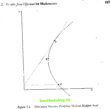 Given a riskfree asset with return Rj the minimum-variance portfolio with expected return Hp will be the solution to the constrained optimization min о/Пи, (5-2.20) subject (о As in the prior problem, we form the I .agrangian function /., differentiate it with respect to w. set the resulting equations to zero, and then solve for w. For the Lagrangian function we have c L = wOw + S - w/i - (1 - Щ) (5.2.22) Differentiating /. with respect to w and setting the result equal to zero, we haVC 2nw-*0i-tyi> = 0. (5-2.23) Combining (5.2.23) with (5.2.21) we have StZ31 n-(/i - K/i). (5-2.24) (M-/{/t)ir(M- /t) Note that we can express u, as a scalar which depends on die mean of p limes a portfolio weight vector which does not depend on )>, where u.A = (5.2.25) H- ЦсУГГц- lift) (5.2.21)) ш = - R,t). (5.2.27) Thus with a riskfree asset all minimum-variance portfolios are a combination of a given risky asset portfolio with weights proportional to wand the riskfree asset. This portfolio of risky assets is called the tangency portfolio and has weight vector fTv/i- lift). (5.2.28) i.il (/t - 11,i) We use the subscript ij lo identify the tangency portfolio. Equation (5.2.28) divides the elements of w by their sum to get a vector whose elements sum to one, that is, a portfolio weight vector. Figure 5.2 illustrates the set of minimum-variance portfolios in the presence of a riskfree asset. With a riskfree asset all efficient portfolios lie along the line from the riskfree asset through portfolio /. The expected excess return per unit risk is useful lo provide a basis for economic interpretation of tests of the CAPM. The Sharpe ratio measures this quantity. For any asset or portfolio a, the Sharpe ratio is defined as the mean excess return divided by the standard deviation of return, ~ Rf si-, = ---. (5.2.2.)) In Figure 5.2 the Sharpe ratio is the slope of the line from the riskfree return ill/, 0) lo the portfolio (/( , cj ). The tangency portfolio </ can be characterized as the portfolio with ihe maximum Sharpe ratio of till portfolios of risky assets. Testing the mean-variance efficiency of a given portfolio is equivalent lo lesling whether the Sharpe ralio of that portfolio is the maximum of the set of Sharpe ratios ol all possible portfolios. 5.3 Statistical Framework for Estimation and Testing Initially we use the assumption that investors can borrow and lend al a riskfree rale ol return, and we consider the Sharpe-I.intner version ol the (АРМ. Then, we climinaic this assumption and analyze the Black version. 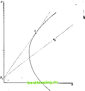 Figure 5.2. Minimum-Variance Portfolios With Riskfree Asset 5.3.1 Sharpe-Lintner Version Define Z, as an (Д/xl) vector of excess returns for N assets (or portfolios of assets). For these N assets, the excess returns can be described using the excess-return market model: Z, = a + (3Z, , + €, (5.3.1) E[e ] = 0 (5.3.2) E[6,e, ] = S (5.3.3) E[Zm,] = iim, Е[(2, ,-/хи)2] = al (5.3.4) Cov[Z, e,] = 0. (5.3.5) /3 is the (iVxl) vector of betas, ZM is the time period t market portfolio excess return, and a and c, are (/Vx 1) vectors of asset return intercepts and disturbances, respectively. As will be the case throughout this chapter wk have suppressed the dependence of a, /3, and e, on the market portfolio or its proxy. For convenience, with the Sharpe-Lintner version, we redefine /1 to refer to the expected excess return. 1 2 3 4 5 6 7 8 9 10 11 12 13 14 15 16 17 18 19 20 21 22 23 24 25 26 27 28 29 30 31 [ 32 ] 33 34 35 36 37 38 39 40 41 42 43 44 45 46 47 48 49 50 51 52 53 54 55 56 57 58 59 60 61 62 63 64 65 66 67 68 69 70 71 72 73 74 75 76 77 78 79 80 81 82 83 84 85 86 87 88 89 90 91 92 93 94 95 96 97 98 99 100 101 102 103 |