Altci natively, if we assume tliat the mean and variance of simple returns It ate in, and л;, respectively, then under the lognormal model the mean and variance of >;, are given by

КIill = log

\ar(i ] = log

in, + 1

(1.4.15)

(1.4.1с.)

The lognormal model has the added advantage of not violating limited liability, since limited liability yields a lower bound of /его on (I + A ), which is satisfied by (1 + H ) = < when r is assumed to be norma!.

The lognormal model has a long and illustrious history, beginning with the dissertation of the French mathematician Louts Bachelier (1900), which contained the mathematics of Brownian motion and heat conduction, live years prior to Einsteins (1905) famous paper. For other reasons that will become apparent in later chapters (see, especially, Chapter 9), the lognormal model has become the workhorse of the financial asset pricing literature.

But as attractive as the lognormal model is, it is not consistent with all the properties of historical stock returns. At short horizons, historical returns show weak evidence of skewness and strong evidence of excess kurtosis. The skewness, or normalized third moment, of a random variable ( with mean ц and variance я - is defined by

S[() на E

U - ИГ

The kuitmis, or normalized fourth moment, of с is defined bv

K\(] = к

(1.4.17)

(1.4. is)

The normal distribution has skewness equal to zero, as do all other symmetric distributions. The normal distribution has kurtosis equal to 3, but fat-taileddistributions with extra probability mass in the tail areas have higher or even infinite kurtosis.

Skewness and kurtosis can be estimated in a sample of data by constructing the obvious sample averages: the sample mean

l.-i. tnees, Kebinis, and Comjmuniling

the sample variance

the sample skewness

and the sample kurtosis

In large samples of normally distributed data, the estimators S and К are normally distributed with means 0 and 3 and variances 6/T and 24/ T respectively (see Stuart and Ord [1987,Vol. 1]). Since 3 is the kurtosis of the* normal distribution, sample excess kurtosis is defined to be sample kurtosis less 3. Sample estimates of skewness for daily US stock returns tend to be negative for stock indexes but close to zero or positive for individual stocks. Sample estimates of excess kurtosis for daily US stock returns are large and positive for both indexes and individual stocks, indicating that returns have more mass in the tail areas than would be predicted by a normal distribution.

Stable Distributions

Early studies of stock market returns attempted to capture this excess kurtosis by modeling the distribution of continuously compounded returns as a member of the stable class (also called the stable Pareto-lJvy or stable Pare-tian), of which the normal is a special case.3 The stable distributions arc a natural generalization of the normal in that, as their name suggests, they are stable under addition, i.e., a sum of stable random variables is also a stable random variable. However, nonnormal stable distributions have more probability mass in the tail areas than the normal. In fact, the nonnormal stable distributions are so fat-tailed that their variance and all higher moments are infinite. Sample estimates of variance or kurtosis for random variables with

l tic French probabili.it Pan! Levy (1924) was perhaps the first lo initiate a general investigation of stable distributions and provided a complete characterization of them through their 1оц-< haiactrristic functions (see below). I.evy (192.r>) also showed that the tail probabilities ol stable distributions approximate those of the Parclo distribution, hence the term stable l\ueio-l.evy or stable Paretian distribution. For applications lo financial asset returns, see l l;illlx-rKand Conecles (1974); Fama (1965); Fama and Roll (1971); Fieliu (1976); Fieliu and Ko/cll (198,4); Oranger and Mornenstern (1970); Hageniian (1978); Hsu, Miller, and Wirhern (1974); Mandelbrot (1%S); Mandelbrot and Taylor (19li7); Officer (1972); Samuetson (1967, 1976); Siuiknwit/ and needles (1980); and Tucker (1992).

0.40

Manual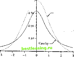

Figure 1.2. Comparison of Stable and Normal Density Functions

these distributions will not converge as the sample size increases, hut will tend to increase indefinitely.

Closed-form expressions for the density functions of stable random variables are available for only three special cases: the normal, the Cauchy, and the Bernoulli cases.4 Figure 1.2 illustrates the Cauchy distribution, with density function

/(*) = -

(1.4.23)

7T у* + (X - &)г

In Figure 1.2, (1.4.23) is graphed with parameters <S = 0 and у = 1, and it is apparent from the comparison with the normal density function (dashed lines) that the Cauchy has fatter tails than the normal.

Although stable distributions were popular in the 1960s and early H)70s, they are less commonly used today. They have fallen out of favor partly be- cause they make theoretical modelling so difficult; standard finance theory

4 However,-Levy (1925) derived the following explicit expression lor the logarithm of the characteristic function <p(t) ol any stable random variable A: logv>(<) s logE* v) = Hi -ИРП - #5gii(l)taii(oor/2)), where (a./i.S.y) are the lour parameters that characterize each stable distribution. S € (-00, 00) is said to be the location parameter, /1 e (-00. cxd) is the ikrvmtss iniUx, у e (0,oo) is the ualt parameter, and a € (0.2 is the expontnt. When a = 2, ihe stable distribution reduces to a normal. As or decreases from 2 to t), the tail areas ol tin stable distribution become increasingly latter than the normal. When a e (1. 2), the stable distribution has a finite mean given by S, but when or e (0. 1 J, even the mean is infinite. The parameter p measures the symmetry of the stable distribution; when 0 = 0 the distribution is symmetric, and when p > 0 (or p < 0) the distribution is skewed lo the right (or left). When P = 0 and a = 1 we have the Cauchy distribution, and when a = 1/2, /i = I, i = 0, ami у = 1 we ItaviVtbe Bernoulli distribution.

almost always requires finite second moments of returns, and often finite higher moments as well. Stable distributions also have some counterfac-lual implications. First, they imply that sample estimates of the variance and higher moments of returns will tend to increase as the sample size increases, whereas in practice these estimates seem lo converge. Second, they imply that long-horizon returns will be just as non-normal as short-horizon returns (snee long-horizon returns are sums of short-horizon returns, and these distributions are stable under addition). In practice the evidence lor non-normality is much weaker for long-horizon returns than for short-horizon returns.

Recent research tends instead lo model returns as drawn from a fat-tailed distribution with finite higher moments, such as the С distribution, or as drawn from a mixture of distributions. For example ihe return might be conditionally normal, conditional on a variance parameter which is itself random; ihen the unconditional distribution of returns is a mixture of normal distributions, some with small conditional variances that concentrate mass around the mean and others with large conditional variances that put mass in the tails of the distribution. The result is a fat-tailed unconditional distribution with a finite variance and finite higher moments. Since all moments are finite, the Central Limit Theorem applies and long-horizon returns will tend 10 be closer to the normal distribution than short-horizon returns. Il is natural to model the conditional variance as a time-series process, and we discuss this in detail in Chapter 12.

An Empirical Illustration

Table 1.1 contains some sample statistics for individual and aggregate stock returns from the Cenier for Research in Securities Prices (CRSP) lor 1962 to 1994 which illustrate some of the issues discussed in the previous sections. Sample moments, calculated in the straightforward way described in (1.4.19)-(1.4.22), are reported for value- and equal-weighted indexes of stocks listed on the New York Stock Exchange (NYSE) and American Stock Exchange (AMEX), and for ten individual stocks. The individual stocks were selected from market-capitalization deciles using 1979 end-of-year market capitalizations for all stocks in the CRSP NYSE/AMEX universe, where International Business Machines is the largest deciles representative and Continental Materials Corp. is the smallest deciles representative.

Panel A reports statistics for daily returns. The daily index returns have extremely high sample excess kuriosis, 34.9 and 26.0 respectively, a clear sign of fat tails. Although the excess kuriosis estimates for daily individual stock returns arc generally less than those for die indexes, they are still large, ranging from 3.35 to 59.4. Since there are 8179 observations, the standard error for the kuriosis estimate under the null hypothesis of normality is 24/8179 = 0.054, so these estimates of excess kurtosis are overwhelmingly

/. tlllKKllU tlu/l

statistically significant. The skewness estimates are negative (or the daily index returns, -1.33 and -0.93 respectively, hut generally positive for the individual slock returns, ranging from -0.18 to 2.25. Many of the skewness estimates are also statistically significant as the standard error under the null hypothesis of normality is /0/8179 = 0.027.

Panel В reports sample statistics for monthly returns. These are considerably less leplokuilic than daily returns-the value- and equal-weighted CRSP monthly index returns have excess kurtosis of only 2.42 and 4.14, respectively, an order of magnitude .smaller than the excess kurtosis of daily returns. As there are only 390 observations the standard error for the kurtosis estimate is also much larger, 0.248. This is one piece of evidence that has led researchers to use fat-tailed distributions with finite higher moments, for which the Central Limit Theorem applies and drives longer-horizon returns towards normality.

1.5 Market Efficiency

The origins of the Efficient Markets Hypothesis (EMH) can be traced back at least as far as the pioneering theoretical contribution of Bachelier (190(1) and the empirical research of Cowles (1933). The modern literature in economics begins with Samiielson (1905), whose contribution is neatly summarized by the title of his article: Proof that Properly Anticipated Prices Fluctuate Randomly / In an inlormatioiially efficient market-not to be confused with an allocationally or Pareto-cfficient market-price changes must be unforecaslablc if they are properly anticipated, i.e., if they fully incorporate the expectations and information of all market participants.

Fama (1970) .summarizes this idea in his classic survey by writing: Л market in which prices always fully reflect available information is called efficient. Famas use of quotation marks around the words fully reflect indicates that these words are a form of shorthand and need to be explained more fully. More recently, Malkiel (1992) has offered the following mote explicit definition:

A capital market is said to be efficient if it fully and correctly reflects all relevant information in determining security prices. Formally, the market is said to be efficient with respect to some information set ... if security prices would be unaffected by revealing that information to all participants. Moreover, efficiency with respect to an information set

Bernstein (19921 discusses the с ouu ihutious ul Bachelier, Cowles, Samuctson, ami mam other eartv authots. tin- .uncles tepcintcd in l.o (1996) include some o( the most important papers in litis literature.

Market EJpriency

Table 1.1. Stork market returns, 1962 to 1994.

Standard Excess

Security Mean Deviation Skewness Kurtosis Minimum Maximum

Panel A: Daily Returns

.Summary statistics for daily and monthly returns (in percent) of CRSP equal- and value-weighted stock indexes and ten individual securities continuously listed over the entire sample period from July 3, 1962 to December 30, 1994. Individual securities are selected to represent slocks in each size decile. Statistics are defined in (1.4.I9)-(1.4.22).

... implies that it is impossible to make economic profits by trading on the basis of [that information set].

Malkiels first sentence repeats Famas definition. His second and third sentences expand the definition in two alternative ways. The second sentence suggests that market efficiency can be tested by revealing information (o