7. Iresenl-Value Relations

сап lead lo statistical ilillii ullics in finite samples. An alternative approach is to assume dial ilie dynamics of die dala are well described by a simple lime-series model; long-liori/oii properties can then be imputed from the shoil-iun model talliei than estimated directly. In the variance-bounds literature, this is die approach of I.eRoy and Porter (1981). These authors note thai a variance-hounds list does not require observations of the perfect-lorcsighl price [>; itself; it merely requires an estimate of the variance of/л*, which can be obtained from a univariate time-series model for dividends. West (1988b) develops a variant of this procedure.

To see how ibis approach can work, suppose that one observes (he complete vector of state variables x, used by market participants, and that x, follows a vet tor autoregressive (VAR) process. Any VAR model can be written in first-order form by augmenting the stale vector with suitable lags of the original variables, so without loss of generality we write:

x,u = Ax, + ,+ ,. (7.2.18)

1 lere A is a matrix of VAR coefficients, and en\ is a vector of shocks to the VAR. We have dropped constants for simplicity; one can think of the state vector as including demeaned variables.

Equation (7/2.1S) implies that inulliperiod forecasts of the stale vector x, can be formed by inairix multiplication:

K,x,m, = A+,x,. (7.2.19)

Plus makes il easy to calculate (he long-horizon forecasts that determine prices in (7.1.22) and (7.1.23), or die revisions of long-horizon forecasts thai determine returns in (7.1.25) and (7.i.20).

Vector Aitlinegiessions and Irice Volatility

As a first example, suppose thai the slate vector includes the slock price /i, as its lirsl element and the dividend d, as its second element, while the remaining elements are other relevant forecasting variables. We define vectors el = I 1)0 ... 0 and c.2 = 0 1 0 ... 0]. These vectors pick out the first element (pt) and the second element (</,) from the stale vector x,. Using these definitions and equations (7.1.22), (7.1.23), and (7.2.19). the dividend component of die slock price is

Il, = (1 ~,i)]TVc-2A lx, = (I - p)e2A(I - рАГх,- (7.2.20)

Ihe slock price itself is /<, - clx so the expecled-reluru component of the slock price is the difference- between the Iwo. If expected relurns are

7.2. I resen I- Value Relations a ml US Slock Irice Behavior

constant, then p, = p which imposes the restriction

el = (l-p)e2A(I-pA)-1 (7.2.21)

on the VAR system. This can be tested using a nonlinear Wald test.16

So far we have assumed that the vector x, includes all the relevant vari- j ables observed by market participants. Fortunately this very strong assump- I tion can be relaxed. Even if x, includes only a subset of the relevant in- . formation, under the constant-expected-return null hypothesis the stock price should still equal the best VAR forecast of the discounted value of future dividends as given on the right-hand side of (7.2.21). Intuitively, when the null hypothesis is true the stock price perfectly reveals investors information about the discounted value of future dividends. Another way to see the same point is to interpret the restriction (7.2.21) as enforcing the unforecastability of multiperiod stock returns. If multiperiod returns are unfbrecastable given investors information, they will also be unfore-castable given any smaller set of information variables, and thus the VAR test of (7.2.21) is a valid test of the null hypothesis.

One can also show that (7.2.21) is a nonlinear transformation of the restrictions implied by the unforecastability of single-period stock returns. In the VAR system the single-period stock return is unforecastable if and only if

el(I-pA) = (1-p)e2A, (7.2.22)

which is obtained from (7.2.21) by postmultiplyingeach side by (I-pA). The economic meaning of this is that multiperiod returns are unforecastable if and only if one-period returns are unforecastable. However Wald test statistics are sensitive to nonlinear transformations of hypotheses; thus Wald tests of the VAR coefficient restrictions may behave differendy when the restrictions are stated in the infinite-horizon form (7.2.21) than when they are stated in the single-period form (7.2.22). An interesting question for future research is how alternative VAR test statistics behave in simple models of time-varying expected returns such as the AR(1) example developed in this chapter.

An important caveat is lhat when the constant-expected-return null hypothesis is false, the VAR estimate of pj, will in general depend on the information included in the VAR. Thus one should be cautious in interpreting VAR estimates that reject the null hypothesis. As an example, consider an updated version of the VAR system used by Campbell and Shiller (1988a) which includes the log dividend-price ratio and the real log dividend growth rale. These variables are used in place of ihe real log price and log dividend

for details see Campbell and Shiller (19R7, l.IRRa.b). Campbell and Shiller also show how to test oilier models of expected slock returns in the VAR framework.

282 7. Present-Value Relations

oq t .

i I860 1880 1900 1920 1940 1960 1980 2000

figure 7.1. Log Ileal Stock Price and Dividend Series, Annual US Data, 1H72 lo 1994

in order to ensure that the VAR system is stationary. The system is estimated with four lags using annual data from 1871 to 1994. Figure 7.1 shows the real log stock price as a solid line and the real log dividend as a dashed line. Both series have been demeaned so that the sample mean in the Figure is zero. The two lines tend to move together, but the movements of the log stock price arc larger than those of the log dividend; thus the price-dividend ratio is procyclical and the dividend-price ralio is countercyclical. Figure 7.2 again shows the demeaned real log slock price as a solid line, hut now the dashed line is the demeaned VAR estimate of pdi, the present value of future dividends. Because the real log dividend is close to a random walk, the \YVR estimate of рл, is close to d, itself anil thus the variation in /v, is larger than that in рц. Figure 7.3 shows the log dividend-price ratio as a solid line a>id the log ratio of dividend to p,u as a dashed line.17 The present-value njiodcl with constant discount rales explains very little of the variation in slock prices relative to dividends, i While this general conclusion is robust, the smoothness of/),/, is sensitive to the specification of die VAR system, ln a low-order system with four lags

These series have not been demeaned; the level <>f the dividend-price ratio can lie reeov-etled Iron! the figure by exponentiating the plotted solid line.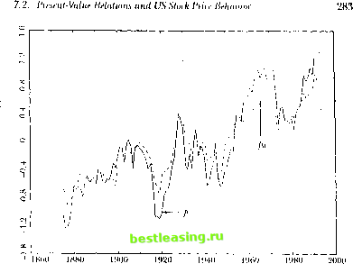

Figure 7.2. Lug Real Stock Price and Estimated Dividend Oanponent, Annual LIS Data, lS76lo 1994

or fewer, />, moves closely with d,. As one increases the lag length towards ten lags, pltl becomes much smoother and more like a trend line. The same thing happens if one adds to the VAR system a ratio of price to a 10-year or 30-year moving average of earnings, as suggested by Campbell and Shillcr (1988b). There appears to be some long-run mean-reversion in dividend growth which is captured by these expanded VAR systems.

In conclusion, the VAR approach strongly suggests that the slock market is too volatile lobe consistent with the view thai slock prices are optimal forecasts of future dividends discounted at a constant rate. Some VAR systems suggest that the optimal dividend forecast is close to the current dividend, others that die optimal dividend forecast is even smoother than the current dividend; neither type of system can account for the tendency of slock prices lo move more than one-for-one with dividends.1 Strictly speaking, however, once the null hypothesis pt = р,ц is rejected, any interpretation

Rarsky and De Long (199.$) /joint out thai slink /nice behavior could be rationalized if there were a unit-root component in dividend growth, bin they do uoi present any direct econometric evidence lor such а сош/юпеш. Donaldson and Kainslra (1990) argue that a nonlinear dividend forecasting model delivers more volatile loretaSLs ol long-run future dividends. This remains an active research area.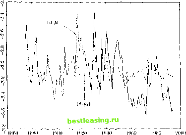

Figure 7.3. Log Dividend-Price ltalio and Estimated Dividend (.omjionent. Annual US dala. IH7(Uo IWI

of lite behavior of /;,/, is conditional on Ihe information variables included in the VAR.

Vector A utoregressions and Return Volatility

A common criticism o( volatility tests, which applies equally to VAR systems including prices and dividends, is that the lime-series process driving dividends may not be stable through time.11 Fortunately it is possible to analyze the variability of siock returns without modeling the dividend process. Consider a slate vector x, whose lirsl element is the one-period stock return and whose other elements are relevant forecasting variables for returns. With this system the unexpected stock return becomes

rul - F [ = еГе,+ 1. (7.2.23)

The Miidigli.ini Millci tlii-пгщ savs ill.il linn-value inasiini/atiiiii In managers dues пш rt him rain tin- loini <>l dividend nil it v. 1 .t-liiii.iiin ( Ml.ll) uses litis to argue that the smchasiic process describing dividends is llulikclv m In- slablc.

Recall that the revision in expectations of all future slock returns, n t+i, is defined as

1.:t+i = E

2> i+i+>

This becomes

rj ,+i = elYp>A>eM = elpA(I - pA) e,+).

(7.2.24)

From (7.1.26) the revision in expectations of future dividends, f)d,i+i, can be treated as a residual:

iu.i+i = -ЕДг,+ ,]) + >7г +1 = el(l-fpA(I-pA) 1)e(+i.

As a concrete example, consider an updated version of the system estimated by Campbell (1991) in which the state vector has three elements; the real stock return (r,), the log dividend-price ratio (д,), and the level of the stochastically detrended short-term interest rate (хц). Using monthly data over the period 1952:1 to 1994:12, the estimated first-order VAR for these variables, with asymptotic standard errors in parentheses, is

( r+1 \ *u+i /

(7.2.25)

The matrix in (7.2.25) is a numerical example of the VAR coefficient matrix A. The R2 statistics for the three regressions summarized in (7.2.25) are 0.040, 0.996, and 0.537, respectively, indicating a modest degree of fore-castability for monthly stock returns.20

- As the roellirieni estimates suggest, the log dividend-price ratio has a root extremely close to unity in this sample period. Although there are theoretical reasons for believing lhat the log dividend-pi ire ralio is stationary, and imil-root tests reject a unit root over long sample periods in US data, the persistence of Ihe log dividend-price ratio does lead lo inference problems in the VAR system. I lodrick (1УУ2) is a careful Monte Carlo study of these problems.