hir Benchmark Portfolio

Wc can restate these results in a more familiar way by introducing the idea of a benchmark portfolio. Wc first augment the vector of risky assets with an artificial unconditionally riskless asset whose return is l/M - I. Recall that ijvc have proceeded under the assumption lhat no unconditionally riskless ;jisscl exists; but if it were to exist, its return would have to be 1/Л7 - I. We lhen define the benchmark portfolio return as

- m;(m)

Ri (m) = --=--1. (8.1.1(1)

It is straightforward lo check that this return can be obtained by forming a I portfolio of the risky assets and the artificial riskless asset, and that il satisfies the condition (8.1.8) on returns. Problem 8.1 is to prove that R/ has the f llowing properties:

(PI) Rt,t is mean-variance efficient. That is, no other portfolio has

smaller variance and the same mean.

(P2) Any stochastic discount factor M,(M) has a greater correlation with /4i than with any other portfolio. For this reason Rit, is sometimes referred to as a maximum-coirelation portfolio (see Brccdcn, Gibbons, and I.ilzcnbcrgcr [1989]).

(P3) All asset relurns obey a beta-pricing relation with the benchmark portfolio. That is,

Ф-vjr1)]= р {т ]-{ш-]))- ,81л7)

where вц = Cov[/i; /4,]/VatUu ]. When an unconditional zero-beta asset exists, then it can be substituted into (8.1.17) to get a conventional beta-pricing equation.

Two further properties are useful for a geometric interpretation of the I Ianscn-Jagannathan bounds. Consider Figure 8.1. Panel (a) is the familiar mean-standard deviation diagram for asset returns, with die mean gross return plotted on the vertical axis and the standard deviation of return on the horizontal. Panel (b) is a similar diagram for stochastic discount factors, with the axes rotated; standard deviation is now on the vertical axis and mean on the horizontal. This convention is natural because in panel (a) wc think of assets second moments determining their mean returns, while in panel (b) we vary the mean stochastic discount factor exogenously and trace out the consequences for the standard deviation of the stochastic

l+lt

(A/)

(l>)

Figure 8.1. <a) Mean-Standard Deviation Ihiiginni pir Asset ltd urns; lb) Implicit Standard Deviation-Mean Diagmiu for Stochastic Discount todins

discount factor. In panel (a), the feasible sel of risky asset relurns is shown. Wc augment litis with a riskless gross return I W on die vertical axis; the iiiiniiimin-variance set is then die tangent line from l/Л/ lo the feasible set of risky assels, and die reflection of the langcni in the vertical axis. Properly (PI) means that the benchmark portfolio return is in (he niiiiiniuni-vai iance sel. It plots on the lower branch because its positive correlation with the stochastic discount laclor gives it a lower mean gross return than I/Л/.

fi. Intertemporal Ftjuitil/rium Models

Wc can now stale two more properties:

(P4) Ilierati.iorstaiHlaulrlevialionio gross meaii lor the henchniark >orilolii) salislics

l/ЛТ-КЦ + lh, 1 -- (8.1.18)

But the right-hand side ol° this equation is just the slope ol the tangent line in panel (a) olFigure 8.1. As explained in Chapter 5, this slope is the maximum Sharpe ratio lor the set of assets.

(P5) The ralio of standard deviation to mean for the benchmark portfolio gross return is a lower bound on the same ratio for the stochastic discount factor. That is,

< МШ)] (8 , 1С))

F-ll +/U ~ Y.[M,W)]

lroperlies (14) and (IT)) establish that the stochastic discount factor in panel (h) must lie above the point where a ray from the origin, with slope equal to die maximum Sharpe ratio in panel (a), passes through the vertical line at M. As we vary Л7, we trace out a feasible region for the stochastic discount fat lor in panel (b). This region is higher, and thus more restrictive, when the maximum Sharpe ratio in panel (a) is large for a variety of mean stochastic discount factors M. A set of asset return data with a high maximum Sharpe ratio over a wide range of Л1 is challenging for asset pricing theory in the sense that il requires the stochastic discount factor to be highly variable. By looking at panel (a) one can see that such a data set will contain portfolios with very different mean returns and similar, small standard deviations. A leading example is the set of returns on US Treasury hills, which have differences in mean returns that are absolutely small, hut large relative to the standard deviations of bill returns.

The above analysis applies to returns themselves; the calculations are somewhat simpler if excess returns are used. Writing the excess return on asset /over some reference asset /((not necessarily riskless) as /. = R - Rkl, and the vector ol excess returns as Z the basic condition (8.1.4) becomes

0 = F.Z,A/,]. (8.1.20)

Proceeding as before, wc form МШ) = Л? + (Z, - V.\Z,\Vpj-r where the tilde is used to indicate that j3 is defined with excess returns. We find that fijj = fi (- /WF.Z,), when- il is the vai iauce-cov.ui.UH e matrix of excess returns. Il follows that the lower bound on the variance of the stochastic (list omit fat tor is now

V;ivl Л1,*(Л7)I = AT F.Z,ST~F.Z,. (8.1.21)

8.1. The Stochastic Discount Factor

If we have only a single excess return /. then this condition simpli to Var [M*(M)] = M2(E[u])2/Var[z,],or

crtMM)] = ЕЩ M o[4]

This is illustrated in Figure 8.2, which has the same structure as Figure 8.1, Now the restriction on the stochastic discount factor in panel (b) is that it should lie above a ray from the origin with the same slope as a ray from the origin through the single risky excess return in panel (a).

Implications of Nonnegalivity

So far we have ignored the restriction that M, must be nonnegative. Hansen and Jagannathan (1991) show that this can be handled fairly straightforwardly when an unconditionally riskless asset exists. In this case the mean of M, is known, and the problem can be restated as finding coefficients a that define a random variable

M,*+ = ((4 + R,)a)+, (8.1.23)

where X+ = max(X, 0) is the nonnegative part of X, subject to the constraint

F.[(t + R()M,*+] = E[(z + R,)((<. + R,)a)+] = t. (8.1.24)

In the absence of the nonnegativity constraint, this yields the previous solution for the case where there is an unconditionally riskless asset. With the nonnegativity constraint, it is much harder to find a coefficient vector a that satisfies (8.1.24); Hansen and Jagannathan (1991) discuss strategies for transforming the problem to make the solution easier. Once a coefficient vector is found, however, it is easy to show that M+ has minimum variance among all nonnegative random variables M, satisfying (8.1.8). To see this, consider any other M, and note that

ЕЩМ,+ ] = E[M,((t-fR,)a)+]

> aE[(t + R,)M,l

= aE[(t4-R,)M;+] = E[(M,*+)2]. (8.1.25)

But if Е[Л4,М + ] > Е[(М;+)2], then Е[М;-] > Е[(М;+)2] since.the correlation between these variables cannot be greater than one.

The above analysis can be generalized to deal with the more realistic case in which there is no unconditionally riskless asset, by augmenting the return vector with a hypothetical riskless asset and varying the relurn on this asset. This introduces some technical complications which are discussed by Hansen and jagannathan (1991).

Л02 A Intertemporal Hijiiilibriui/i Models

l + Z

<т(Л()

(1>)

Figure 8.2. (a) Mean-Standard Deviation Diagram for a Single Excess Asset lieturn; (b) Implied Standard Deviation-Mean Diagram (or Stochastic Discount Factors

A First Look al the Equity Premium Puzzle

The Hansen-Jagannalhan approach can he used to understand the well-ktlown equity premium puzzle of Mehraaud Irescotl (1985).2 Mehra and Itlcscott argue that the average excess return on the US slock market-the

j Cochrane ami Hansen (НТО) approach ihe eiiiily premium puzzle from this point of view. Koclierlakola (1990) surveys the large literature on the puzzle.

8.1. The Stochastic Discount Factor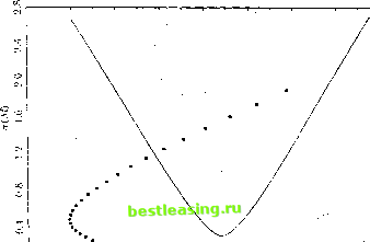

о I...........

° 0.80 0.84 0.88 0.92 0.96 1.00 1.04 1.08 1.12

Figure 83. Feasible Region [or Stochastic Discount Fin Iocs Implied hy Annual US Dala, 1891 lo IW4

equity premium-is loo high to be easily explained by standard asset pricing models. They make this point in ihe context of a tighlly parametrized consumption-based model, but it can be made more generally using the excess-return restriction (8.1.22). Over the period 1889 to 1994, the annual excess simple return on the Standard and Poors slock index over commercial paper has a standard deviation of 18% and a mean of 13%.s Thus the slope of the rays from the origin in Figure 8.2 should be 0.06/0.18 = 0.33, meaning thai the standard deviation of the stochastic discount factor must be at least 33% if it has a mean of one. As we shall sec in the next section, the standard consumption-based model with a risk-aversion coefficient in the conventional range implies that the stochastic discount factor has a mean near one, but an annual standard deviation much less than 33%.

vrhe return on six-month eonunrrcial paper, tolled over in anuary and July, is used instead ol a Treasury hill return because Trcasiuy bill dala are not available in the early pan of this long sample period. Mehra and I Vest oil (1985) splice together routine icial paper and Treasury bill rales, whereas bete we use coiunicrrial paper tales lliiouglmut the sample period lot consistency. The i hoic e of shoi t-lenn tales makes little dilleiem e lo the lesulls. Table 8.1 below gives some sample uioment.s for log assel returns, but the moments slated here are lor simple returns.