technology over the past three decades. Although a detailed discussion ol derivative pricing models is hcyond the scope of this text-there are many other excellent sources such as Cox and Rubinstein (1985), Dull (1993), and Mellon (1990)-we do provide brief reviews of Brownian motion in Section 9.1 and Merlons derivation of the Black-Scholes formula in Section 9.2 for convenience.

Ironically, although pricing derivative securities is often highlv computation-intensive, in principle it leaves very little room for traditional statistical inference since, bv (he verv nature of the no-arbitrage pricing paradigm, there exists no error term to be miniini/ed and no corresponding statistical lluclualious to contend with. After all, if an options price is determined exactly-without error-as some (possibly lime-varying) combination of prices of other traded assets, where is the need for statistical inference? Methods such as regression analysis do not seem lo play a role even in the application of option pricing models to dala.

However, there arc al least two aspects of the implementation of derivative pricing models that do involve statistical inference and we shall focus on them in this chapter. The first aspect is the problem of estimating the parameters of continuous-time price processes which are inputs for parametric derivative pricing tin inul.is. We use the qualifier parametric in describing the derivative pricing formulas considered in this chapter because several nonparametric approaches lo pricing derivatives have recently been proposed (see, for example, Aii-Sahalia 11992), Ait-Sahalia and l.o 11995], Hutchinson, l.o. and Ioggio 199 lj, and Rubinstein 1994).- We shall consider nonparaiuclric derivative pricing models in Chapter 12, and focus on issues surrounding parametric models in Section 9.3.

The second aspect involves the pricing of path-dependent derivatives by Monte Carlo simulation. A derivative security is said lo be path-dependent if its payoff depends in some way on the entire path of the underlying assets price during the derivatives life, for example, a put option which gives the holder lite right to sell the underlying asset al its average price-where the average is calculated over the life of the option-is path-dependent because the average price is a fuiii lion of the underlying assets entire price path. Although a few analytical approximations for pricing path-dependent derivatives do exist, by far the most effective method for pricing them is by Monte Carlo simulation. This raises several issues such as measuring tin- accuracy of simulated prices, deteimining the number of simulations required for a desired level of accuracy, and designing the simulations to

In toniiasl lii ilie li.iililiuii.il ).u .niii-l i и ,i iii i i.ii Ii in uliiili ihe price process nl the iindt-i lying asset is lnIK sjiei ilu-ii iii in .i liniie number of unknown parameters, e.g., a loguor-inal ilitliisiuii \\j111 unknown iliilt am! volatility paiaiuclcis, a uniiparautcti ic approach does HiW specilv ihe priie pint ess explicitly anil attempts ti> infer il from ihe data untler suitable regularity ciiiiiliiinns.

make the most economical use of computational resources. We turn to

these issues in Section 9.4.

9.1 Brownian Motion

For certain financial applications it is often more convenient to model prices as evolving continuously through time rather than discretely at fixed dates. For example, Mertons derivation of the Black-Scholes option-pricing foij-mula relies heavily on the ability to adjust portfolio holdings continuously in-time so as to replicate an options payoff exactly. Such a replicating portfoj-lio strategy is often impossible to construct in a discrete-time setting; hencej pricing formulas for options and other derivative securities are almost always, derived in continuous time (see Section 9.2 for a more detailed discussion).*

9.1.1 Constructing Brownian Motion

The first formal mathematical model of financial asset prices-developed by Bachelier (1900) for the larger purpose of pricing warrants trading on the Paris Bourse-was the continuous-time random walk, or Brownian motion. Therefore, it should not be surprising that Brownian motion plays such a central role in modern derivative pricing models. This continuous-time process is closely related to the discrete-time versions of the random walk described in Section 2.1 of Chapter 2, and we shall take the discrete-time random walk as a starting point in our heuristic construction of the Brownian motion.1 Our goal is to use the discrete-time random walk to define a sequence of continuous-time processes which will converge to a continuous-time analog of the random walk in the limit.

The Discrete-Time Random Walk

Denote by a discrete-time random walk with increments that.take on only two values, Д and - Д:

!Д with probability л u u им- . , (9U)

- Д with probability л = 1 - тг,

where e /, is IID (hence pk follows the Random Walk 1 model of Section 2.1.1 of Chapter 2), and po is fixed. Consider the following continuous-time process / О, 6 [0, T], which can be constructed from the discrete-time process

There are two notable exceptions: the equilibrium approach of Rubinstein (1976), and the binomial opiion-pi icing model of Cox, Ross, and Rubinstein (1979). For a more rigorous derivation, see Billingsley (1968, Section 37).

5Д

9. Derivative Iricing Models

4Д- -°

ЗД - - > --° ---°

2Д - --< --

1Д- -°

o4-?-1-1-1-1-г---i--i

0 h 2Л ЗА 4Л bit 6Л T = nh

I Figure 9.1. Sample Path of a Discrete-Time IbrntUm Walk

{pk), k= 1,.... n as follows: Partition the time interval [0, 7] into pieces, each of length Л = T/n, and define the process

MO = ft/M = Pimm, t e [0.71, (0.1.2)

where [x] denotes the greatest integer less than or equal to x. p (t) is a rather simple continuous-time process, constant except at times I - Ith, к = 1,..., n (see Figure 9.1).

Although MO is indeed a well-defined continuous-time process, it is still essentially the same as the discrete-time process pi, since it only varies at discrete points in time. However, if we allow n to increase without bound while holding T fixed (hence forcing Л to approach 0), then the number of points in [0, T] at which p (l) varies will atso increase without bound. If, at the same time, we adjust the step size Д and the probabilities ir and n appropriately as n increases, then p (t) converges in distribution to a well-defined nondegenerate continuous-time process p(t) with continuous sample paths on [0, 7].

To see why adjustments to Д, n, and я are necessary, consider the mean and variance of p {T):

ПрЛП) = п(л-л)Д . .. (9.1.3)

. Varl/> (7 )1 = 4нтгггД2. (9.1.4)

As n increases willjoui bound, the mean and variance of/*в(Т) will also i -

9.1. Ilrtmtnian Motion

crease without bound if Д, тг, and n are held fixed. To obtain a well-defined and nondegenerate limiting process, we must maintain finite moments for p (T) as n approaches infinity. In particular, since we wish lo obtain a continuous-time version of the random walk, we should expect the mean and variance of the limiting process p(T) to be linear in T, as in (2.1.5) and (2.1.6) for the discrete-time random walk. Therefore, we must adjust Д, л, and тг so that:

/(7Г-7Г)Д = - (Л-7Г)Д -> u7

4П7Г7ГД2 == - 47Г7ГД- -> CllT,

and this is accomplished by selling: 1 /, /V

;r = [1--

:i \ a

The adjustments (9.1.7) imply thai the step size decreases as n increases, bin at the slower rate of 1 A/n or Jli. The probabilities converge to j, also at the rate of Jli, and hence wc write:

jr = l + o-JTi), я = 1 + о(Ул), Д = 0{sfJi). (9.1.Н)

where O(sffi) denotes terms that are of the same asymptotic order as s/h? Therefore, as n increases, the random walk p (T) varies more frequently on [0, 7], but with smaller step size Д and with tip-step and down-step probabilities approaching j.

:A function /(/i) is said lo be ot the same asymptotic older as £{1,)-denoted !>y /(/i) - (HgOO)-if tile following relation is satisfied:

(I < 111!) - < OO.

A-ll gtll)

A function /(/i) is said to lie of;smaller asymptotic otdci as r;(/i)-denoted liy /(/i) ~ (£(/, )) if

r f{h) о

lllll - = 0.

/1-11 Itt/l)

Some examples of asyinptolii order relations are

h - ii[J1i). Mr - u(Jii). bs/Ji + Ir - OtJli). I,-Mr ~ (Hh).

(9.1.5) (9.1.6)

Д = oV/i.

(9.1.7)

The Continuous Time l.imil

By callidaliug the tuoiiicnt-gi-ui-rating (unction of/* (/) and taking its limit as approaches inliiiiiy, it may he shown that ilie (lisirihittion of p(T) is normal with mean /(/and variance a~T\ thus p (T) converges in distribution lo a M(p T. ci-Г) random variable.

In fail, a much stronger notion o( convergence relates / (/) to p(T), which involves the pnile-diinensinnul distributions (lDOs) of the two stochastic processes. An FDD of a stochastic process pit) is the joint distribution of anv (mile number of observations of the stochastic process, i.e.,

/(/(Л), /(AO...../</, )>, where 0 < l\ < < /, < 7. It can be shown lhat

nil the FDDs of the stochastic process /> (/) (not just the random variable / ( I)) converge to the FDDs of a wcll-dcliucd stochastic process pit). litis implies, for example, that ihe dislrihuiion of p (l) converges to the distribution of /;(/) for all / 6 0, 7] (not just al 7), that the joint distribution of l/ (<>), / (3). / (7) converges to the joint distribution of (/ДО), /;(3). p(7)\, and so on.

In-addition to the uorinaliiy of pi 7), the stochastic process pit) possesses the following three properties:

(Rt) For any /, and such thai ()</,< h < T:

pih) - /(/,) ~- Af(n(h - <i).(T-(f, - /,)). (0.1.9)

(R2) For any I-., f and /., such thai 0 < (i < t-> < h < t.t < 7\ ihe increineni pit*) - p(t\) is statistically independent of the increment pil\)-p(h).

(R3) flu- sample paths of pit) are continuous.

Il is a remarkable fact that (/), which is the celebrated arithmetic Brownian motion or Wiener process, is completely characterized by these three properties. If we set /i = 0 and гт = I, we obtain standard Brownian motion which we shall denote by /1(0. Accordingly, we may re-express p(l) as

pit) = nl + nli(i). I e [0, 71. (9.1.10)

lo develop further intuition for /)(/), consider (he following conditional moments:

F.I/U) I pi Ml = pil ) + iiV-t ) (9.1.11)

Var (/) I pil )\ = n-ii - / ) (9.1.12)

Hie i отпцгш с ill МЯК, i mtjHcH with а им him ,\\ t ontiitmnal t .tHcil light nrw, )\ t .tiled m-iik i шип цок r. a ionvi Mil км ) in <lci i\itij4 .is\ hi ] >m it i< approximations loi ilie siaiisii* al laws ol in.mv iHiiiliin-ai t-Minialoi v Src Hillinslcv (\*M\H) for Itutlici (ItUils.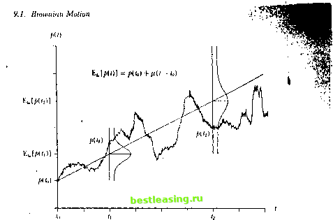

Figure 9.2. Sample Path and Conditional Expectation of a Hwwnian Motion with Drift

Соу[р(1,).р(Ш = Cov[#/,). +/>(/,)] (9.1.13) = Cov[p(tt), p(t2) -p(t,)]

+ Cov[/. ,)./ ( i)] (9.1.14)

= Var[/ (fi)] = (9.1.15)

As for the discrete-time, random walk, the conditional mean and variance of p(l) are linear in t (see Figure 9.2). Properties (B2) and (B3) of Brownian motion imply that its sample paths are very erratic and jagged-if they were smooth, the infinitesimal increment B(t+h)-B(t) would be predictable by B(t)-B(t-h), violating independence. In fact, observe lhat the ratio (B(l+h)-B(l))/hAoe% not converge to a well-defined random variable as h approaches 0, since

ГВ +Л)-В(0 Var -

L л

Therefore, ihe derivative of Brownian motion, B(t), does not exist in the ordinary sense, and although the sample paths of Brownian motion are everywhere continuous, they are nowhere differcntiable.

-. (9.1.16)