show in Section 10.2.1 that historically, movements in short-term interest rates have tended to be larger than movements in longer-term bond yields. Some modified approaches have been developed to handle the more realistic case where short yields move more than long yields, so that there arc nonparallel shifts in the term structure (see Bierwag, Kaufman, and Toevs [1983],Granilo [1984], Ingersoll, Skellon, and Weil [1978]).

Second, (10.1.11) and (10.1.12) give first-order derivatives so they apply only to infinitesimally small changes in yields. Figure 10.4 illustrates the fact that the relationship between the log price and the yield on a bond is convex rather than linear. The slope of this relationship, modified duration, increases as yields fall (a fact shown also in Table 10.1). This may be taken into account by using a second-order derivative. The convexity of a bond is defined as

d2/> i ГУ <+!> i я(я-Н)

Convextty а -Гуту- = -J,- 00.1.13)

find convexity can be used in a second-order Taylor series approximation of the price impact of a change in yield:

1 *ЫУп) dl> , 11 #Pn 1

j lr ~ dYn,Pc l + 2 dYl pj

j = (- modified duration) dYr

J 4- ~ convexity (dYr )2- (10.1.14)

Finally, both Macaidays duration and modified duration assume that ish flows are fixed and do not change when interest rates change. This a: sumption is appropriate for Treasury securities but not for callable securi-ti :s such as corporate bonds or mortgage-backed securities, or for securities w th default risk if the probability of default varies with the level of interest rates. Bymodelling the way in which cash flows vary with interest rates, it is possible to calculate the sensitivity of prices to interest rates for these more complicated securities; this sensitivity is known as effective duration.

ALoglinear Model for Coupon Bonds

The idea of duration has also been used in the academic literature to find approximate linear relationships between log coupon bond yields, holding-period returns, and forward rates that are analogous to the exact relationships for zero-coupon bonds. To understand this approach, start from the

nSce Fabozzi and Fabo .i (11)1)5) Chapters 2H-30, and Fabo/.zi (ltK№) lor a discussion of various methods used try fixed-income analysts to calculate effective duration.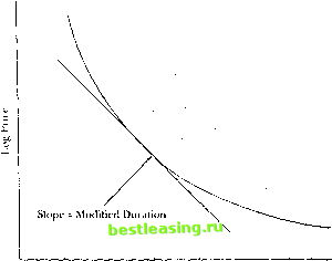

Yield

Figure 10.4. The Price-Yield Itelalioiiship

loglinear approximate return formula (7.1.19) derived in Chapter 7, and apply it lo the one-period relurn rf, .,+ i on an н-pcriod coupon bond:

>. ./+1 ~ h +ppr, .i.ltl -I- (1 - p)c-p . (10.1.15)

Here the log nominal coupon с plays the role of the dividend on stock, but of course it is fixed rather than random. The parameters p and к are given by p = 1/(1 4- exp(c - />)) and As- log(p) - (1 - p) Iog(l/p - 1). When ihe bond is selling al par, then its price is $1 so its log price is zero and p = 1/(14- Q = (1 4- Ff i) l. It is standard to use this value for p, which gives a good approximation for returns on bonds selling close to par.

One can treat (10.1.15), like die analogous zero-coupon expression (10.1.5), as a difference equation in the log bond price. Solving forward lo the maturity date one obtains

P = ХУ-Н!-/>)<- )>. -,-./+i+,!- (10,1.16)

This equation relates the price of a coupon bond lo its stream of coupon payments and the future returns on the bond. Л similar approximation of the

10. Eixed-lnconie Securities

log yield lo maturity у shows thai i( satisfies an equation of the same form:

i=ii

= LLL!/,. + (l -pj.-v ]. (10.1.17)

(!-/>)

Kqnations (10.1.10) and (10.1.17) logclher imply that the /.-period eonpon bond yield satisfies y ((1 -/>)/(! -/> )) E!= /)r,. ;.,+, + ,. finis although there is no exact relationship there is an approximate equality between the log yield to maturity on a coupon bond and a weighted average of the returns on the bond when it is held to maturity.

Equation (10.1.1 1) tells us dial Macaulays duration for a coupon bond is the derivative ol its log price with respect lo its log yield. Equation (10.1.17) gives (his derivative as

* = + (10.1.18)

(l-/i) I - (1+ > )

where the second equality uses p = (1 + !, ,) 1. As noted above, this relation between duration and yield holds exactly for a bond selling at par.

Substituting (10.1.17) and (10.1.18) into (10.1.15), we obtain a loglincar relation between holding-period returns and yields for coupon bonds:

;. . i * 1>. У. > - ( r - *)>. -(IO.t.19)

This equation was first derived by Shiller, Campbell, and Schocnholtz (19H3). Ii is analogous lo (Hi.1.5) for zero-coupon bonds; maturity in thai equation is replaced by duration here, and of course the two equations are consistent with one another for a zero-coupon bond whose duration equals its maturity.

A similar analysis for forward rales shows that the м-pcriod-ahcad 1-pcriod forward rale implicit in the coupon-bearing term structure is

(10.1.20)

Д.я11-Дм

This formula, which is also due to Shiller, Campbell, and Schoenholtz (1983), reduces lo the discount bond formula (10.1.8) when duration equals maturity.

1 Sliillei.l :.ini>l>rlt, .им! S, lim nlu.li/ use !, , instead ol y, i. Out diesc ate equivalent lu the same liisl-iinlei a>iiii\iiiialion used id ileiive (III.I.HI). Iliey .dsn derive liinnnlas relalini; lllillli)eriiid liiildini; lelin lis In virlds.

iti.l. Basic Concepts

409

The classic immunization problem is that of finding a coupon bond or portfolio of coupon bonds whose return has the same sensitivity to srriall interest-rate movements as the relurn on a given zero-coupon bond. Alternatively, one can try to find a portfolio of coupon bonds whose cash flows exactly match those of a given zero-coupon bond. In general, this portfolio will involve shortselling some bonds. This procedure has academic interest as well; one can extract an implied zero-coupon term structure from the coupon term structure.

If the complete zero-coupon term structure-that is, the prices of discount bonds Pi ... P maturing at each coupon date-is known, then it is easy to find the price of a coupon bond as

Pc = PiC+PiC + - + Pnil + Q. (10.1.21)

Time subscripts are omitted here and throughout this section to economize on notation.

Similarly, if a complete coupon term structure-the prices of coupon bonds Pr\ ... P,n maturingateach coupon date-is available, then (10.1.21) can be used to back out the implied zero-coupon term structure. Starting with a one-period coupon bond, Рл = Pt(l + C) so P) = Pci/(1 4- C). We can then proceed iteratively. Given discount bond prices Pi,..., P i, we can find P as

Pn, - P.,-1С - - Pi С = -Чт~С- (Ю.1.22)

Sometimes the coupon term structure may be more-than-complele in the sense that at least one coupon bond matures on each coupon date and several coupon bonds mature on some coupon dates. In this case (10.1.21) restricts the prices of some coupon bonds to be exact functions of the prices of other coupon bonds. Such restrictions are unlikely to hold in practice because of lax effects and other market frictions. To handle this Carleton and Cooper (1976) suggest adding a bond-specific error term to (10.1.21) and estimating it as a cross-sectional regression with all the bonds outstanding at a particular date. If these bonds are indexed i = 1... /, then the regression is .

Pr = P[Q + Р-гС, + + P ,(l 4- Q) + u j = 1... /, (10.1.2?)

where C, is the coupon on the ith bond and n, is the maturity of the iih bond. The regressors are coupon payments at different dates, and the coefficients are the discount bond prices P;,j- 1 N, where N = maxj n, is the longekt coupon bond maturity. The system can be estimated by OLS provided that the coupon term structure is complete and that I > N.

Spline Estimation

In practice the lenn structure of coupon bonds is usually incomplete, and this means that the coefficients in (10.1.23) are not identified without imposing further restrictions. It seems natural to impose that the prices of discount bonds should vary smoothly with maturity. McCulloch (1971, 1975) suggestslhat a convenient way to do this is to write P, regarded as a function of maturity P(n), as a linear combination of certain prespecified functions:

pn = P( ) = I+]£qj5(n). (10.1.24)

McCulloch calls P(n) the discount function. The fin) in (10.1.24) arc known functions of maturity n, and the я; arc coefficients to be estimated. Since P(0) = 1, wc must have fii)) = 0 for all j.

i Substituting (10.1.24) into (10.1.23) and rearranging, we obtain a regression equation

П, = jajXij + Ui, i=l.../, (10.1.25)

where П, = Pr, , - 1 - Qn the difference between the coupon bond price arid the undiscounlcd value of its future payments, and X1; = f,ini) + C\jS21=] fj{l). Like equation (10.1.23), this equation can be estimated by 01.S, but there arc now only J coefficients rather than A/.lr

I A key question is how to specify the functions fin) in (10.1.24). One simple possibility is to make Pin), the discount function, a polynomial. To do this one sets f(n) = n>. Although a sufficiently high-order polynomial can approximate any function, in practice one may want to use more parameters to fit the discount function at some maturities rather than others. For example one may want a more flexible approximation in maturity ranges where many bonds are traded.

To meet this need McCulloch suggests that P(n) should be a spline function.1K An rth-ordcr spline, defined over some finite interval, is a piece-wise rth-ordcr polynomial with r- 1 continuous derivatives; its rth derivative is a step function. The points where the rth derivative changes discontin-uously (including the points at the beginning and end of the interval over which the spline is defined) are known as knot points. If there are К knot

The bond pricing errors arc unlikely lo be homoskedastic. McCulloch argues that the standard deviation of t/, is proportional to the bid-ask spread for bond i, and lints weights each observation by the reciprocal of its spread. This is not required for consistency, bill may improve the efficiency of the estimates.

Suits, Mason, and Chan (HI78) give an accessible introduction to spline methodology.

points, there are A. - 1 subintervals in each of which the spline is a polynomial. The spline has К - 2 + r free parameters, r for the first subiulerval and 1 (that determines the unrestricted nh derivative) lor each of the A-2 following subintervals. McCulloch suggests (hat (he knot points should be chosen so that each subiulerval contains an equal number of bond maturity dales.

II forward rales are to be continuous, the discount function must have al least one continuous derivative. Hence a quadratic spline, estimated by McCulloch (1971), is the lowest-order spline that can lit the discount function. II we require that the forward-rale curve should also be continuously difler-entiable, then we need to use a cubic spline, estimated by McCulloch (1975) and others. McCullochs papers give ihe rather complicated formulas for the functions fin) that make Iin) a quadratic or cubic spline.17

7 rev Effects

OLS estimation of (10.1.25) chooses the parameters a, so that the bond pricing errors иi are uncorrelated with the variables a;, that define the discount function. If a sufficiently flexible spline is used, then the pricing errors will be uncorrelated with maturity or any nonlinear function of maturity. Pricing errors may, however, be correlated with the coupon rale which is die other defining characteristic of a bond. Indeed McCulloch (1971) found that his mode! tended to underprice bonds that were selling below par because of iheir low coupon rates.

McCulloch (1975) attributes this to a lax effect. US Treasury bond coupons are (axed as ordinary income while price appreciation on a coupon-bearing bond purchased at a discount is taxed as capital gains. If the capital gains lax rate r is less than the ordinary income tax rate r (as has often been the case historically), then this can explain a price premium on bonds selling below par. For an investor who holds a bond to maturity the pricing formula (10.1.21) should be modified to

> , = U - rsU - l\ )\P(n) + (1 - т)С J2 () (Ю.1.26)

The spline approach can be modified to handle tax effects like that in (10.1.26), al the cost of some additional complexity in estimation. Once tax effects are included, coupon bond prices must be used to construct the variables X on the right-hand side of (10.1.25). This means dial the bond pricing errors arc correlated with the regressors so die equation must be

.Adams and van Dc-venter (19У4) argue for the use of a lourth-ordet spline, with the cubic term omitted, in order lo maximize- the smoothness ol ihe lorwaid-rate riitvc, where smoothness is tie-lined to be minus the average squared second cleiivaiive ol the loi ward-rate curve with respect to maturity.