It). Itxed-Iucoine Securities

estimated by insiiumcntal variables raiber than simple OI.S. l.ii/enberger and Rolfo (1981) apply a lax-adjusied spline model of ibis sort lo bond market data front several different countries.

Tlie lax-adjusted spline model assumes thai tlie same tax rates are relevant for till bonds, flic model caiinol handle clientele effects, in which differently taxed investors specialize in different bonds. Schaefer (1981, 1982) suggests that clientele effects can be handled by first finding a set of tax-efficient bonds for an investor in a particular tax bracket, then estimating an implied zero-coupon yield curve from those bonds alone.

Nonlinear Mullets

Despite the flexibility of the spline approach, spline functions have some unappealing properties. First, since splines are polynomials they imply a discount function which diverges as maturity increases rather than going to zero as required by theory. Implied forward rates also diverge rather than converging lo any fixed limit. Second, there is no simple way lo ensure that the discount function always declines with maturity (i.e., that all forward rates are positive). The forward curve illustrated in Figure 10.1 goes negative at a maturity of 27 years, and this behavior is not uncommon (see Shea I I981). These problems are related lo the fact thai a flat zero-coupon yield curve implies an exponentially declining discount function, which is not easily approximated by a polynomial function. Since any plausible yield curve llatlens out al the long end, splines are likely lo have difficulties with longer-maturity bonds.

These difficulties have led some authors lo suggest nonlinear alternatives to the linear specification (10.1.21). One alternative, suggested by Vasicck and Kong (1982), is to use an exponential spline, a spline applied to a negative exponential transformation of maturity. The exponential spline has the desirable property that forward rates and zero-coupon yields converge to a fixed limit as maturity increases. More generally, a Hat yield curve is easy lo lit with an exponential spline.

Although die exponential splint is appealing in theory, it is not clear that il performs better than the standard spline in practice (see Shea [1985]). The exponential spline does not make it easier lo restrict forward rates to be positive. As lor its long-maturity behavior, il is important lo remember dial forward rales cannot be directly estimated beyond the maturity of the longest coupon bond; they can only be identified by restricting the relation between long-horizon forward rates and shorter-horizon forward rates. The exponential spline, like the standard spline, fits the observed maturity range llexibly, leaving ihe liiniling forward rale and speed of convergence lo ibis rale lo be determined more by the restrictions of the spline than by any characteristics of the long-horizon data. Since the exponential spline involves nonlinear estimation of a parameter used to transform maturity, il is

10.2. interpreting tlie Verm Structure oj Interest Rates

more difficult to use than the standard spline and this cost may outweigh the ; exponential splines desirable long-horizon properties. In any case, forward rate and yield curves should be treated with caution if they are extrapolated beyond the maturity of the longest traded bond.

Some other authors have solved the problem of negative forward rates by restricting the shape of the zero-coupon yield curve. Nelson and Sjiegel (1987), for example, model the instantaneous forward rate at maturity n as the solution to a second-order differential equation with equal roots: f(n) - /Jo + ySi exp(-an) -\-anB.zexp(-an). This implies that the discount function is double-exponential:

P(n) = exp[-A, n + {B.+ &)(! - exp(-an))/a - и/}2exp(-o>n)p.

This specification generates forward-rate and yield curves with a desiable range of shapes, including upward-sloping, inverted, and hump-shaped. Svensson (1994) has developed this specification further. Other recent work has generated bond-price formulas from fully specified general-equilibrium models of the term structure, which we discuss in Chapter 11.

10.2 Interpreting the Term Structure of Interest Rates

There is a large empirical literature which tests statements about expected-return relationships among bonds without deriving these statements from a fully specified equilibrium model. For simplicity we discuss this literature assuming that zero-coupon bond prices are observed or can be estimated from coupon bond prices.

10.2.1 The Expectations Hypothesis

The most popular simple model of the term structure is known as the expectations hypothesis. We distinguish the pure expectations hypothesis (PEH) (PEH), which says that expected excess returns on long-term over short-term bonds are zero, from the expectations hypothesis (EH), which says that expected excess returns are constant over time. This terminology is due to Lutz (1940).

Different Forms of the Pure Expectations Hypothesis

We also distinguish different forms of the PEH, according to the time horizon over which expected excess returns are zero. A first form of the PEH equates the one-period expected returns on one-period and п-period bonds. The one-period return on a one-period bond is known in advance to be (1 + )[,), so this form of the PEH implies

0 + Y ) = E,[l+ R J+l] = (\ + Y, ) E,[(\ + У м+1)-( -,)], (10.2.1)

Table 10.2. Means and stundnnl deviations o( term sh ui hue v/n/iddes.

Long hoiiil maturities are measured in months, tor each variable the table reports the sample mean and sample standard deviation (in parentheses) using monthly data over the period I.lolM-HKM :2. The units are annualized percentage points. The midei lying dala are zero-coupo.-i bond yields from McCulloch and Kwon (100:1}.

Var( r ., + i - Ун J, which measures the quantitative importance oil lie Jensens Inequality effect in a lognormal homoskedaslic model.

Table 10.2 reports unconditional sample means and standard deviations for several term-structure variables over the period 1952:1 to 1991:2. All dala are monthly, but are measured in annualized percentage points; dial is, the raw variables are multiplied by 1200. The first row shows the mean and standard deviation of excess returns on it-niontli zero-coupon bonds over one-month bills. The mean excess return is positive and rising with maturity at lirsl, but il starts lo fall al a maturity of one year and is even slightly negative for ten-year zero-coupon bonds.

This pattern can be understood by breaking excess returns into the two components on the right-hand side of equation (10.2.5): die yield spread (y i - To) between -period and one-period bonds, and -(к - 1) limes the change in yield (y -i.i+i - v, ) on the -period bond. Interest rales of all fixed maturities rise during the sample period, as shown in die second row olTable 10.2 and illustrated foronc-nionih and ten-year rales in Figure 10.5. Al the short end of the term structure this effect is offset by the decline in maturity from n to н- 1 as the bond is held for one month; thus the change

fable 10.2 is an expanded version of a table shown in (.ampbcll (n(-,), Ihe numbers given heie are slightly dillerent from the numbers in that paper beiaiisc the sample period used in that paper was 1051:1 to 10*. 10:2, all hough it was erroneously I epoi led lo be HI52:1 lo l.l.ll:2.

wh< re the second equality follows from die definition of holding-period return and the fact that (1 4- Yul) is known at time t.

A second form of the PEH equates the n-period expected returns on one-period and n-pcriod bonds:

(1+ / ,) = E/[(l + K/)(I + r*i./+i)...(l + y l+ ,)]. (10.2.2)

Here (1 + Y ,) is the n-pcriod relurn on an n-period bond, which equals the expected return from rolling over one-period bonds for n periods. It is straightforward to show that if (10.2.2) holds for all n, it implies

s (i + y > ,)-T = K.Il + Ku+H-!]. (Ю.2.3)

Under this form of the РЕМ, the ( - l)-period-ahead one-period forward rate, equals the expected (n - l)-period-ahcad spot rate.

lit is also straightforward to.show that if (10.2.2) holds for all n, il implies

! (1+Г ,) = (l+K )E,[(l + r -i.,+ i) ]. (Ю.2.4)

But (10.2.4) is inconsistent with (10.2.1) whenever interest rates arc random. The problem is that byjenscns Inequality, the expectation of the reciprocal of a random variable is not the reciprocal of the expectation of that random variable. Thus the pure expectations hypothesis cannot hold in both its one-period form and its n-period form.

One can understand this problem more clearly by assuming that interest rales are lognormal and homoskedastic and taking logs of the one-period PEH equation (10.2.1) and the n-period РЕМ equation (10.2.4). Noting that from equation (10.1.5) the excess one-period log return on an n-period bond is

r<u+l-yu = (y i->!/)-( -l)(? -i./+1 -y.n), (10.2.5)

equation (10.2.1) implies that

E[r . +i-yu] = -(l/2)Var[, .,H -j ], (10.2.6) while (10.2.4) implies that

E[r ,+ i-yu] = (1/2) Var[ +, -y ]. (10.2.7)

The difference between the right-hand sides of (10.2.6) and (10.2.7) is

,HCox, Ingersnll, and Ross (l.)Kla) make this point very clearly. They also argue lhat in continuous time, only expected equality of instantaneous returns (a model corresponding to (Itl.U.t)) is consistent with the absence ol arbitrage. But McCulloch (1МУ.Ч) has shown thai this result depends on restrictive assumptions and does not hold in general.

1 111

III. Fixed-Income See amies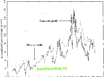

l.irifi I.niu i. ir> i.170 Hi7r> i.mo i.mr> I.i.io i.ior>

Figure 10.5. Sliarl- anil Long-Term Interest Hates 1952 lo 1991

in yield (> -/+ - y i), shown in the third row of Table 10.2, is negative for short bonds, contributing positively to their return.20 At the long end orthe term structure, however, the decline in maturity from n to n - 1 is negligible, and so die change in yield (vm-i.i+i - v /) is positive, causing capilal losses on long zero-coupon bonds which outweigh the higher yields offered by these bonds, shown in die fourth row of Table 10.2.

The standard deviation of excess returns rises rapidly with maturity. If excess bond returns are while noise, then the standard error of the sample mean is the standard deviation divided by the square root of the sample size (400 months). The standard error for n = 2 is only 0.03%, whereas the standard error for и = 120 is 1.71%. Thus the pattern of mean returns is imprecisely estimated at long maturities.

The standard deviation of excess returns also determines the size of the wedge between the one-period and ji-pcriod forms of the pure expectations hypothesis. The difference between mean annualized excess returns under (10.2.0) and (10.2.7) is only 0.0003% for и = 2. It is still only 0.11% for

- Investors whii sect, lo (nolil lioni tins It-iKtrnrv ol boiiil yields to lull as inaliiritv shrinks an* sail! to lie rilling ihr yield rnrvr.

10.2. Interpreting the Term Structure of Interest Rates

n = 24. But it rises to 1.15% for n - 120. This calculation shows that the differences between different forms of the PEH are small except for very long-maturity zero-coupon bonds. Since these bonds have the most imprecisely estimated mean returns, the data reject all forms of the PEH at the short end of the term structure, but reject no forms of the PEH at the long end of the term structure. In this sense the distinction between different forms of the PEH is not critical for evaluating this hypothesis.

Most empirical research uses neither the one-period form of the PEH (10.2.6), nor the и-period form (10.2.7), but a log form of the PEH that equates the expected log returns on bonds of all maturities:

E[r .,+t -> ] = 0. (10.2.8)

This model is halfway between equations (10.2.6) and (10.2.7) and can be justified as an approximation to either of them when variance terms are small. Alternatively, it can be derived directly as in McCulloch (1993).

Implications of the Ij>g Pure Expectations Hypothesis

Once the PEH is formulated in logs, it is comparatively easy to state its implications for longer-term bonds. The log PEH implies, first, that the one-period log yield (which is the same as the one-period return on a one-period bond) should equal the expected log holding return on a longer гг-period bond held for one period:

yu = E,[r +I]. (10.2J.9)

Second, a long-term n-period log yield should equal the expected sum of n successive log yields on one-period bonds which are rolled over {or n periods:

Уш = (!/ )£ E,[y- +,]. <10.2.10)

Finally, the (n - l)-period-ahead one-period log forward rate should equal the expected one-period spot rate (n - 1) periods ahead:

= E,[y ,+ -t]. (10.2.1J1)

This implies that the log forward rate for a one-period investment to be made at a particular date in the future should follow a martingale:

f,a = E,[y. + ] = E,[E,+1[y,.,+,;]] = £,[/ + ]. X10.2.12)

If any of equations (10.2.9), (10.2.10), and (10.2.11) hold for all n and /, then the other equations also hold for all n and Л Also, if any of these