/ /. lerm-Structure Models

coefficients) and tin- role of die stale variables in determining excess bond returns (measured by I lie Bn coefficients). The system is particularly easy to understand in the single-factor case. Here К - 1, we can drop the к subscripts, and (II.2.II) becomes

; (, HJ>r (11.2.15)

Equation (I 1.2.15) says that each row of the matrix С is proportional to each other row, and the eocftieicnlsof proportionality arc ratios of Л* coefficients. Note that the rank of the matrix С could be less than K; for example, it is /его in a homoskedaslic model with A. state variables because in such a model the coefficients Bkn are /его for all ft and n.

Latent-variable models of the form (11.2.14) or (11.2.15) have been applied to financial data by Campbell (1987), Gibbons and Ferson (1985), and Hansen and Hodrick (198.!). They can be estimated by Generalized Method of Moments applied to the system of regression equations (11.2.13). I lesion (1992) points out that one can equivalently estimate a system of instrumental variables regressions of excess returns on A. basis excess returns, where the elements of h, are the instruments.

Л key issue is how to choose instruments h, that satisfy (11.2.10) (orthogonality of instruments and bond pricing errors) and (11.2.11) (stale variables linear in the instruments). In an affme-yield model without bond pricing errors, bond yields and forward rates are linear in the stale variables; hence the state variables are linear in yields and forward rates. This property survives the addition of normally distributed bond pricing errors. Thus ii is natural to choose yields or forward rates as instruments satisfying (11.2.11).

To satisfy (11.2.10), one must be more specific about the nature of the bond pricing errors. The error in a bond price measured at time 1 affects both the lime / bond yield and the excess return on the bond from / to /4-1. Hence yields and forward rates measured at time / are not likely to be orthogonal lo errors in excess bond returns from / to / 4- I. If the bond price errors are uncorrelated across time, however, then yields and forward rates measured al lime / - I will be orthogonal to excess bond return errors from ( to / -I 1; and if (he bond price errors are uncorrelated across bonds, then one can choose a set of yields or forward rates measured at different maturities than those used for excess returns. Stambaugh (1988) applies both these strategies to monthly data on US Treasury bills of maturities two lo six months over the period 1959:3 lo 1985:11. He finds strong evidence against a model with one state variable and weaker evidence against a model with two stale variables. I lesion (1992) studies a more recent period, 1970:2 lo 1988:5, and a data set including longer maturities (0, 12, 30, and 00 months) and finds linle evidence against a model with one slate variable.

/1.2. Fitting Term-Structure Models to the Data

Evidence on the Short-Rate Process

If one is willing to assume that there is negligible measurement error in the short-term nominal interest rate, then time-series analysis of short-rate behavior may be a useful first step in building a nominal term-structure model. Chan, Karolyi, Longstaff, and Sanders (1992) estimate a discrete-time model for the short rate of the form

E,[<?,+1] = 0, E,[ ?+)] = ayi,. (11.2.17)

yi.t+i-Ум = + РУи + £,+ ), (11.2.16)

where

r n v ri(+)J

This specification nests the single-factor models we discussed in Section 11.1; the homoskedaslic model has у = 0, while the square-root model has у - 0.5. It also approximates a continuous-time diffusion process for the instantaneous short rate r(t) of the form dr - (p0 + p\r)dt + arY dB. Such a diffusion process nests the major single-factor continuous-time models for the short rate. The Vasicek (1977) model, for example, has у = 0; the Cox, Ingersoll, and Ross (1985a) model has у = 0.5, and the Brennan and Schwartz (1979) model has у = l.B

Chan et al. (1992) estimate (11.2.16) and (11.2.17) by Generalized Method of Moments. They define an error vector with two elements, the fir$t being yiJ+i ~{l+P)yu-a and the second being (yt +i - (1 + P)yn - ot) j-агУи These errors are orthogonal to any instruments known at time /; ja constant and the level of the short rate y\, are used as the instruments. \n monthly data on a one-month Treasury bill rate over the period 1964:6 tb 1989:12, Chan et al. find that a and P are small and often statistically insignificant. The short-term interest rate is highly persistent so it is hard to reject the hypothesis lhat il follows a random walk. They also find that y; is large and precisely estimated. They can reject all models which makc у < 1, and their unrestricted estimate of у is about 1.5 and almost two standard errors above 1. j

To understand these results, consider the case where a = P = 0, so the short rate is a random walk without drift. Then the error term in (11.2.16) isjust the change in the short rate y\ +\-yu, and (11.2.17) says that the expectation of the squared change in the short rate, E,[(jti,+i - уц)21 = aiy\yt. Equivalently,

/+1 - Ун /и

(11.2.18)

so when the change in the short rale is scaled by the appropriate power of the short rale, it becomes homoskedastic. Figures 11.1a through d illustrate

Note however lhat (11.2.10) and (11.4.17) do not nest the Pearson-Sun model.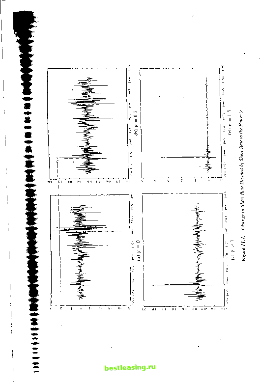

the results of (ban elal. by plotting changes in short rates scaled by various powers of short rales. The figures show (yi.i+i - >i,)/(v[() for у - 0, 0.5, 1, and 1.5, using the dala of McCulloch and Kwon (1003) over die period 1052:1 to 1091:2. Over die period since 1904 studied by Chan et al., it is striking how the variance of the seiies appears lo stabilize as one increases у from 0 to 1.5.

These results raise two problems for single-factor affine-yield models of the nominal term structure. First, when there is no mean-reversion in the short rate, forward rates and bond yields may rise with maturity initially, but Ihey eventually decline with maturity and continue to do so forever. Second, singlc-faclorafliiic-yield models require that у = 0or0.5 in (I 1.2.17). The estimated value of 1.5 lakes one outside the tractable class of alline-yield models and forces one lo solve the terni-slriiclure model numerically.

There is as yet no consensus about how lo resolve these problems. Ail-Saludia (1996b) argues that existing parametric models are too restrictive; he proposes a nonparametric method for estimating the drift and volatility of the short interest rate. He argues that the short rate is very close to a random wab when it is in the middle of its historical range (roughly, between 4% and 17%), but that it mean-reverts strongly when it gels outside this range. Chan et al. miss ibis because their linear model does not allow mean-reversion lo depend on the level of the interest rate. Ail-Sahalia also argues thai intcrcsl-ralc volatility is related to the level of the interest rate in a more complicated way than is allowed by any standard model. His most general parametric model, and ihe only one he docs not reject.statistically, has die short interest rate following the diffusion dr = (ft + ft i + ft2 + ft/)/ + ( *o + a\ -f a-,rY)dR. He estimates у to be about 2, but the other parameters of the volatility function also play an important role in determining volatility.

Following Hamilton (1989), an alternative view is dial die short rate randomly switches among different regimes, each of which has its own mean and volatility parameters. Such a model may have mean-reversion within each regime, but die short rate may appear lo be highly persistent when one averages dala from different regimes. If regimes with high mean parameters are also regimes with high volatility parameters, then such a model may also explain the apparent sensitivity of interest rale volatility lo the level of the interest rate without invoking a high value of у. Figures 1 l.la-d show that no single value of у makes scaled interest rate changes homoskedastic over the whole period since 1952; the choice of у = 1.5 works very well for 1964 lo 1991 but worsens hcleroskedasticity in die 1950s and early 1960s.7 Thus al least some regime changes arc needed lo fit the dala, and il may be thai a model with у = 0 or у = 0.5 is adequate once regime changes

Although this is not shown in the ligutcs, the у ~ 1.Г> model .tlso hrc.iks down in the I.HIOs.

11. Term-Structure Models

are allowed. Gray (1996) explores lhis possibility but estimates only slirrlnly lower values ol у than Chan et al., while Naik and l.ee (1994) solve lor bond and bond-option prices in a regime-shift model with у = 0.

Brenner, llarjes, and Kroner (I99(i) move in a somewhat dilfercnt direction. They allow for GARCH effects on interest rate volatility, as described in Section 12.2 of Chapter 12, as well as the level effect on volatility described by (11.2.17). They replace (11.2.17) by V.,[(f+l] = afy\r and erf = ш + Of + </>T/i a standard GARCH(1,1) model. They find that a model with у = 0.5 (its the short rale series quite well once GARCH effects are included in the model; however they do not explore the implications of this for bond or bond-option pricing.

Cross-Sectional Restrictions on the Term Structure

So far we have emphasized the time-series implications of affme-yield models and have ignored their cross-sectional implications. Brown and Dybvig (19K0) and Brown and Schaefer (1994) take the opposite approach, ignoring the models time-series implications and estimating all the parameters from the term structure of interest rates observed at a point in time. If this procedure is repealed over many time periods, it generates a sequence of parameter estimates which should in theory be identical for all time periods but which in practice varies over time. The procedure is analogous to the common practice of calculating implied volatility by inverting the Black-Scholes formula using traded option prices; there too the model requires dial volatility be constant over lime, but implied volatility lends lo move over time.

Of course, bond pricing errors might cause estimated parameters to shift overtime even il true underlying parameters are constant. But in simple term-structure models there also appear to be some systematic dilfciences between the parameter values needed to fit cross-sectional term-structure data and the parameter values implied by the time-series behavior of interest tales. These systematic differences are indicative of inisspccification in the models. To understand the problem, we will choose parameters in the single-factor homoskedaslic and square-root models to lit various simple moments of the data and will show lhat the resulting model does not match some other characteristics of the data.

In the homoskedaslic single-factor model, the important parameters of the model can be identified by considering the following four moments of the data:

Conj Yi,. vi ..i I = ф

11.2. Fitting Term-Structure Models to the Data

lim K[r .,+1 - yii] = lim E[/ - Yn]

ЕЫ = A -p V72. (11.2.19)

The fust-order autocorrelation of the short rate identifies the autoregressive parameter ф. Given ф, the variance of the short rate then identifies the innovation variance a2. Given ф and a1, the average excess return on a very long-term bond, or equivalently the average difference between a very long-term forward rate and the short rate, identify the parameter/). Finally, given ф, a2, and fi, the mean short rate identifies д.

In the zero-coupon yield data of McCulloch and Kwon (1993) over the period 1952 to 1991, the monthly first-order autocorrelation of the short rate is 0.98, implying ф = 0.98. The standard deviation of the short rate is 3.004% at an annual rate or 0.00255 in natural units, implying or = 0.00051 in natural units or 0.610% at an annual rate.

In the data there is some discrepancy between the average excess return on long bonds, which from Table 10.2 is negative at -0.048% at an annual rate for n = 120, and the average slope of the forward-rate curve, which is positive at 1.507% at an annual rate when measured by the difference between a 60-120 month forward rate and the 1-month short rate. The difference occurs because interest rates rose over the period 1952 to 1991; stationary term-structure models force the true mean change in interest rates to be zero, but an increase in interest rates in a particular sample rjan make the sample mean excess return on long bonds negative even when the sample mean slope of the forward-rate curve is positive. The valueiof fi required to lit the average slope of the forward-rate curve is -122. The implied value for ц. - o2/2, expressed at an annual rate, is 7.632%.

The difficulty with the homoskedastic single-factor model is that with these parameters the average forward-rate term-structure curves very gradually from its initial value to its asymptote, as shown by the dashed line in Figure 11.2. The sample average forward-rate curve over the 1952 to 19,91 period, shown by the solid line in Figure 11.2, rises much more steeplyjat first and then (lattens out at about five years maturity. i

This problem arises because the theoretical average forward-rate curye approaches its asymptote approximately at geometric rate ф. One coud match the sample average forward-rate curve more closely by choosing! a smaller value of ф. Unfortunately this would be inconsistent not only wih the observed persistence of the short rate, but also with the observed pattern of volatility in forward rales. Equation (11.1.14) shows that the standard