This mode! can capture nonlmeai ilies parsimoniously (with a finite, short lag length) when pure nonlineai moving-average or nonlinear autoregressive models fail to do so. (.ranger and Andersen (1978) and Suhha R;>o and Gain (1981) explore bilinear models in detail.

Ilecanise-I .incur Л lodels

Another popular way to lit nonlinear structure is to use pieccwise-linear Ilinclions, as in the first-order threshold autoregression (TAR):

i -1- /<i-vi i + (i if.*,-i < к л, = (12.1.9)

ол. + fi.,x, -i -f c, il .*, i > k.

Here the intercept and slope coefficient in a regression of.*, on its lag v, i depend on the value of v, ) in relation to the threshold к. This mode! can he generalized to higher orders and multiple thresholds, as explained in deiail in long (1983, 1990).

Iiei cwise-linear models also include change-point models or, as thev are known in the economics literature, models with structural breaks. In these models, die parameters arc assumed to shift-typically once-during a fixed sample period, and the goal is to estimate the two sets of parameters as well as the change point or structural break. 1erron (1989) applies ibis technique to macrocconoinic time seiies, and Brodsky (1993) and Caiistcin, Midler, and Siegmund (1991) present more recent methods for dealing with change points, including nonparametric estimators and Bayesian inference.

Change-point methods are very well-established in the statistics and operations research literature, but their application to economic models is not without controversy. Unlike the typical engineering application where a structural break is known to exist in a given dalaset, we can never say with certainty that a structural break exists in an economic time series. And if we think a structural break has occurred because of some major economic event, e.g., a stock market crash, this data-driven specification search can bias our inferences dramatically towards finding breaks where none exist (see, for example. Learner I978 and I.о and MacKinlay [ 1990]).

Markov-Switching Models

fhe Markov-switching model of Hamilton (1989, 1990, 1993) and Sclove (1983a, 1983b) is closely related to the TAR. The key difference is lhat changes in regime are determined not by the level of the process, bill bv an unobserved state variable which is typically modeled as a Markov chain. For example,

1 + ft I */ - I + f I, if S/ = 1

(12.1.10)

...-I-ft.v, i +<=.. if s, = 0

12.1. Nonlinear Structure in Univariate Time Series

where s, is an unobservable two-state Markov chain with some transition probability matrix P. Note the slightly different timing convention in (12.1.10): s, determines the regime at time /, not s,-\. In both regimes, x, is an AR(1), but the parameters (including the variance of the error term) differ across regimes, and the change in regime is stochastic and possibly serially correlated.

This model has obvious appeal from an economic perspective. Changes in regime are caused by factors other than the series we are currently modeling (s, determines the regime, not x,), rarely do we know which regime we are in (s, is unobservable), but after the fact we can often identity which regime we were in with some degree of confidence (st can be estimated, via Hamiltons [1989] filtering process). Moreover, the Markov-switching model does not suffer from some of the statistical biases that models of structural breaks do; the regime shifts are identified by the interaction between the data and the Markov chain, not by a priori inspection of the data. Hamiltons (1989) application to business cycles is an excellent illustration of the power and scope of this technique.

Deterministic Nonlinear Dynamical Systems

There have been many exciting recent advances in modeling deterministic nonlinear dynamical systems, and these have motivated a number of techniques for estimating nonlinear relationships. Relatively simple systems of ordinary differential and difference equations have been shown to exhibit extremely complex dynamics. The popular term for such complexity is the Butterfly Effect, the notion that a flap of a butterflys wings in Brazil sets off a tornado in Texas . This refers, only half-jokingly, to the following simple system of deterministic ordinary differential equations proposed by Lorenz (1963) for modeling weather patterns

x У z

Lorenz (1963) observed that even the slightest change in the starting values of this system-in the fourth decimal place, for example-produces dramatically different sample paths, even after only a short time. This sensitivity to initial conditions is a hallmark of the emerging field of chaos theory. \

This is adapted from the (ilie of Edward l/irenz.s address to the American Association for the Advancement of Science in Washington, D.C., December 1979. See Gleick (1987) for a lively and entertaining laymans account of the emerging science of nonlinear dynamical systems, or chaos theory.

100-x) (12.1.(1)

xz + 2Sx-y (12.1.12)

ху-+Л. (12.1.3)

12. Nonlinearities in Financial Data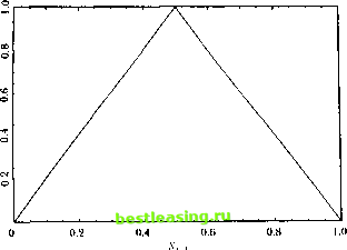

Figure 12.1. Fhe Tent Map

An even simpler example of a chaotic system is the well-known lent map:

x, =

2x, ,

if x,

2(l-x,-,) ifx,-

jq, e (0, 1). (12.1.14)

The tent map can be viewed as a first-order threshold autoregression with no shock f, and with parameters o<i=0, Bi=2, 0(2=2, and ft>= - 2. If x, i lies between 0 and 1, x, also lies in this interval; thus the tent map maps the unit interval back into itself as illustrated in Figure 12.1. Data generated by 1(12.1.14) appear random in lhat they are uniformly distributed on the unjt interval and arc serially uncorrelated. Moreover, the dala also exhibit sensitive dependence to initial conditions, which will be verified in Problem 12.1. Hsieh (1991) presents several other leading examples, while Brock (1986), Holden (1986), and Thompson and Stewart (1986) provide more formal discussions of ihe mathematics of chaotic systems.

Although the many important breakthroughs in nonlinear dynamical systems do have immediate implications for physics, biology, and other hard sciences, the impact on economics and finance has been less dramatic. While a number of economic applications have been considered,2 none are especially compelling, particularly from an empirical perspective.

See, for example, Boldrin and Woodlord (I990), Brock and Sayers (1988), Craig, Kohla.se. and Papell (1991), Day (1983), Crandmnnl and Malgrangc (1986), Hsieh (19ЭД, Keimaii

12.1. Nonlinear Structure in Univariate lime Series

There are two serious problems in modeling economic phenomena as deterministic nonlinear dynamical systems. First, unlike the theory that is available in many natural sciences, economic theory is generally not specific about functional forms. Thus economists rarely have theoretical reasons for expecting to find one form of nonlineai ily rather than another. Second, economists arc rarely able to conduct controlled experiments, and this makes il almost impossible to deduce die parameters of a deterministic dynamical system governing economic phenomena, even if such a system exists and is low-dimensional. When controlled experiments are feasible, e.g., in particle physics, il is possible to recover the dynamics with great precision by taking many snapshots of the system at closely spaced time intervals. This technique, known as a stroboscopic map or a Ioiucare section, has given empirical content to even the most abstract notions of nonlinear dynamical systems, but unfortunately cannot be applied lo non-experimental data.

The possibility that a relatively simple set of nonlinear deterministic equations can generate the kind of complexities we see in financial markets is tantalizing, but it is of little interest if we cannot recover these equations will: any degree of precision. Moreover, the impact of statistical sampling errors on a system with sensitive dependence lo initial conditions makes dynamical systems theory even less practical. Of course, given the rapid pace at which this field is advancing, these reservations may be much less serious in a few years.

12.1.2 Univariate Tests for Nonlinear Structure

Despite the caveats of the previous section, the mathematics of chaos theory has motivated several new statistical tests for independence and nonlinear structure which are valuable in their own right, and we now discuss these tests.

Tests Based on Higher Moments

Our earlier discussion of higher moments of nonlinear models can serve-as the basis for a statistical test of nonlincaiily. Hsieh (1989), for example, defines a scaled third moment:

\\\x, x, , x, ,1

*>(.;> s ,., 2Vu, 02.1.15)

l:[x, lV-

and observes that ip(i, j)=() for all i, f>() for IID data, or data generated by a martingale model that is nonlinear only in variance. 11c suggests estimating

and Uilrien (1993), Iesaran and Poller (1992). .Scheinkman and Lellaion (I9K9). and Scheinkman and Woodlord (1994).

ip(i, j) in the obvious way:

#;./ri *Е*Х-У. (12.1.1(5)

Under the mill hypothesis that уз(/, ))=(>, and with sufficient regularity condi-dons imposed on x, so dial higher moments exist, */Тф(1, j) is asymptotically normal and its variance can be consistently estimated by

V s 11±1±ф, (12.,.17)

I Isielis lest uses one particular third moment of the data, but it is also possible to look al several momcntssimullaneoiisly. The autoregressive polynomial model (12.1.7), for example, suggests that a simple test of nonlinearily in die mean is to regress v, onto its own lags and cross-products of its own lags, and lo lest for the join i significance of die nonlinear terms. Tsay (1986) proposes a test of this sort using second-order terms and M lags for a total of Л/(Л/+1)/2 nonlinear regressors. One can calculate hctcroskedasticily-consistenl standard errors so that the test becomes robust to the presence of nonlinearily in variance.

The Correlation Integral anil tlie Correlation Dimension

To distinguish a deterministic, chaotic process from a truly random process, it is essential to view the data in a sufficiently high-dimensional form. In ihe case of the tent map, for example, the data appear random if one plots x, on the unit interval since x, has a uniform distribution. If one plots x, and x, on the unit square, however, the data will all fall on the tent-shaped line shown in Figure 12.1.

This straightforward approach can yield surprising insights, as we saw in analyzing stork price discreteness in Chapter 3. However it becomes difficult to implement when higher dimensions or more complicated nonlinearities are involved. Crassberger and Irocaccia (1983) have suggested a formal approach to capture this basic idea. Their approach begins by organizing the data (preliltered, if desired, to remove linear structure) into n-hislories x , defined by

= I*. ...i.....x,. (12.1.18)

fhe parameter n is known as the embedding dimension.

The nexl step is to calculate die fraction of pairs of N-histories lhat are close lo one another. To measure closeness, we pick a number l< and i all a pair of п-hislorics v and x close to one another if the greatest absolute dillerence between the corresponding members of the pair is smaller than

iz.l. i\ouuarar Miuuuie in univuntttc i tine .series

k: maxo..... -i x, ,-x, ,j < k. We define a closeness indicator K that is-,

one if the two n-histories are close to one another and zero otherwise:

Ka =

1 if max,=0.....n-t ~ < * щ

0 otherwise.

We define C ,T(ft) to be the fraction of pairs that are close in this sense, in a sample of n-histories of size T:

C r(A) = J==i . (12.1.20)

The correlation integral C (A) is the limit of this fraction as the sample size increases:

Cn(k) = lim C ,TW- (12.1.21)

7-* oo

F.quivalently, it is the probability that a randomly selected pair of n-histories is close.

Obviously the correlation integral will depend on both the embedding dimension n and the parameter к. To see how k can matter, set the embedding dimension n=l so that n-histories consist of single data points, and consider ihe case where the data are IID and uniformly distributed on the unit interval (0,1). In this case the fraction of data points that are within a distance A of a benchmark data point is 2k when the benchmark data point is in the middle of the unit interval (between k and 1-A), but it is smaller when the benchmark data point lies near the edge of the unit interval. In the extreme case where the benchmark data point is zero or one, only a fraction k of the other data points are within k of the benchmark. The general formula for the fraction of data points that are close to a benchmark point b is min(A+6, 2A, A+l-6). As A shrinks, however, the complications caused by this edge problem become negligible and the correlation integral approaches 2A.

Crassberger and Procaccia (1983) investigate the behavior of the correlation integral as the distance measure A shrinks. They calculate the ratio of log C ( A) to log A for small A: j

*- log A

which measures the proportional decrease in the fraction of points that ajre close to one another as we decrease the parameter that defines closeness. In the 111) uniform case with n=\, the ratio log C\(k)/ logk approachps log2A/logA=(log2+logA)/logA=l as k shrinks. Thus izi = 1 for IID uniform data; for small A, the fraction of points lhat are close to one another shrinks at the same rate as A. !