

|
|

|
Промышленный лизинг
Методички
Now consider the heliavior of the correlation integral with higher embedding dimensions n. When ?i=2, we are plotting 2-histories ol the data on a 24limcnsional diagram such as Figure 12.1 and asking what Traction of the 2-historics lie within a square whose center is a benchmark 2-history and whose sides are of length 2k. With uniformly distributed IID data, a fraction 4ft of the data points lie within such a square when the benchmark 2-history is sufficiently far away from the edges of the unit square. Again we handle the edge problem by letting k shrink, and we fmd that the ratio log Oi(k)l log k approaches log 4A2/ log к = (log4-f 2 log /()/ log k = 2 as к shrinks. Thus V2=2 for IID uniform data; for small k, the fraction of pairs of points that are close to one another shrinks twice as fast as k. In general v =jn for IID uniform data; for small k, the fraction of n-historics that are closlc to one another shrinks и times as fast as k. The correlation integral behaves very differently when the data are generated by a nonlinear deterministic process. To see this, consider dala generated by the tent map. In one dimension, such data fall uniformly on the .mil line so we again get tii = l. But in two dimensions, all the data points fall an ihe tent-shaped line shown in Figure 12.4. For small k, the fraction of pairs of points that are close to one another shrinks at the same rate as k so Ti>=l. In higher dimensions a similar argument applies, and v =l for all n wljien data are generated by the tent map. The correlation dimension is defined to be the limit of v as н increases, wbep this limit exists: i; = lim v . (12.1.23) Nonlinear deterministic processes are characterized by finite v. The contrast between nonlinear deterministic data and IID uniform data generalizes to IID data with other distributions, since tf = n for IID data regardless of the distribution. The effect of the distribution averages out because we take each n-hislory in turn as a benchmark n-hislory when calculating the correlation integral. Thus Grassbcrgcr and Procaccia (1983) suggest that one can distinguish nonlinear deterministic data from IID random data by calculating vn for different n and seeing whether it grows with n or converges to some fixed limit. This approach requires large amounts of data since one must use very small k to calculate v and no distribution theory is available for vn. The Brock-Dechert-Scheinkman Test Brock, Dechert, and Scheinkman (1987) have developed an alternative approach lhat is better suited to the limited amounts of data typically available in economics and finance. They show that even when k is finite, if the data are IID then for any n CM = q(/<) . (12.1.24) To understand this result, note that the ratio C n\k\fC {k) can be ink preted as a conditional probability: Pr I max x, , - x, , < k max xv , - .*, ,! < /; r ( .\\ - x,\ < It max .v4 , - д.-, , < Itj . (12.1.25) That is, C +\(k)/C (k) is the probability that two data points are close, given lhat the previous n dala points are close. II the dala are IID, this must equal the unconditional probability that two data points are close, C\(h). Selling C + i(h)/C (k)=Ci(k) for all positive n, we obtain (12.1.24). Brock, Dechert, and Scheinkman (1987) propose ihe BDS test statistic, :г(к) where C j(k) and C\j(lt) arc the sample correlation integrals defined in (12.i. 20), and о т(к) is an estimator of the asymptotic standard deviation of (;..iik)-C\. i (><) . The BDS statistic is asymptotically standard normal under Ihe 111) null hypothesis; it is applied and explained by I Isieh (1989) and Scheinkman and LeBaron (1989), who provide explicit expressions for r} ,(/,). Hsieh (1989) and Hsieh (1991) report Monte Carlo results on the size and power of die BDS statistic in finite samples. While there are some pathological nonlinear models for which C (&)= G(/() as in III) data, the BDS statistic appears to have good power against the most commonly used nonlinear models. Il is important to understand thai it has power against models that are nonlinear in variance but not in mean, as well as models that are nonlinear in mean. Thus a BDS rejection does not necessarily imply that a time-series has a linie-varying conditional mean; il could simply be evidence for a time-varying conditional variance. Hsieh (1991), for example, strongly rejects the hypothesis that common slock returns are IID using die BDS test. He then estimates models oflhc lime-varying conditional variance of returns and gets much weaker evidence against the hypothesis that the residuals from such models are IID. 12.2 Models of Changing Volatility In litis section we consider alternative ways to model the changing volatility of a lime-series г;,+ . Section 12.2.1 presents univariate Autoregressive Conditionally I leteroskcdastic (ARCI I) and stochastic-volatility models, and Section 12.2.2 shows how these may be generalized o a multivariate setting. Section 12.2.3 covers models in which time-variation in (lie conditional mean tt.. isonlineiuities iii / икни nil Dalit is linked to tiinc-vai ration in the conditional variance; these models are nonlinear in both mean and variance. In order to concentrate on volatility, we assume that n,+ ! is an innovation, that is, it has mean /его conditional on time I information. In a finance application, ,;,n might he the innovation in an asset return. We define af to he the time I conditional variance of i/,H or equivalently the conditional expectation of ijjv ,. We assume lhat conditional on time / information, the innovation is normallv distributed: ,/+! ~ (12.2.1) The unconditional variance of the innovation, a2, is just the unconditional expectation of <т,-:! a- = = E[K,[ f+,]] = V,[af}. Thus variability of of around its mean does not change Ihe unconditional variance a1. The variability of nf does, however, affect higher moments of the unconditional distribution of i/,t. In particular, with time-varying erf the unconditional distribution of 1/ 1 has fatter tails than a normal distribution. To show this, we first wi ile: fin = rj,6,+ i. (12.2.2) where tH 1 is an 111) random variable with zero mean and unit variance (as in the previous section) thai is normally distributed (an assumption we did not make in the previous section). As we discussed in Chapter I, a useful measure of tail thickness for the distribution of a random variable у is the normalized fourth moment, or kuriosis, defined by A(y) = E[y /E[f] . Il is well known that the kuriosis of a normal random variable is 3; hence А(еж) = 3. Rut for innovations ;,+ !, we have M)mi> = UHr/fl)- :4f>,]>-<r>fl)- = 3, (12.2.3) 11 his 1 cMtli linlilsiiiilvbri aiisc wc arc working with an inniivaliiin scries ilial lias a coiim.mii (/em) cihhIiiioii.iI mean. Im a series tviili a linic-varyinir conditional inean, ilit- iinconiliiional variance is mil ilie same as ihe сии<iiicliiion.il rxpec tallon ol ilie- coiiiliiiou.il variance. 12.2. Moiiels of Changing Volatility where the first equality follows from the independence of a, and6/+i,andthe inequality is implied by Jensens Inequality. Intuitively, the unconditional distribution is a mixture of normal distributions, some with small variances lhat concentrate mass around the mean and some with large variances that put mass in the tails of the distribution. Thus the mixed distribution has fatter tails than the normal. We now consider alternative ways of modeling and estimating the af process. The literature on this subject is enormous, and so our review is inevitably selective. Bollerslev, Chou, and Kroner (1992), Bollerslev, Engle, and Nelson (19*94), Hamilton (1994) provide much more comprehensive surveys. 12.2.1 Univariate Models Early research on time-varying volatility extracted volatility estimates from asset return data before specifying a parametric time-series model for volatility. Officer (1973), for example, used a rolling standard deviation-the standard deviation of returns measured over a subsampie which moves forward through time-to estimate volatility at each point in time. Other researchers have used the difference between the high and low prices on a given day to estimate volatility for that day (Carman and Klass [1980], Parkinson [1980]). Such methods implicitly assume that volatility is constant over some interval of time. j These methods are often quite accurate if the objective is simply to measure volatility at a point in time; as Merton (1980) observed, if an asset price follows a diffusion with constant volatility, e.g., a geometric Brownian motion, volatility can be estimated arbitrarily accurately with an arbitrarily short sample period if one measures prices sufficiently frequendy.4 Nlson (1992) has shown that a similar argument can be made even when volatility changes through time, provided that the conditional distribution of returns is not too fat-tailed and that volatility changes are sufficiendy gradual. It is, however, both logically inconsistent and statistically inefficient to use volatility measures that are based on the assumption of constant volatility over some period when the resulting series moves through time. To handle this, more recent work specifies a parametric model for volatility first, and then uses the model to extract volatility estimates from the data on returns. ARCH Models A basic observation about asset return data is that large returns (of either sign) tend to be followed by more large returns (of either sign). In other See Section 9.3.2 of Chapter 9. Note however that high-frequency price data are often severely affected by microstructure problems of the sort discussed in Chapter S. This has limited the usefulness of the high-low method of Carman and (Class (1980) and Parkinson (1.№<)). 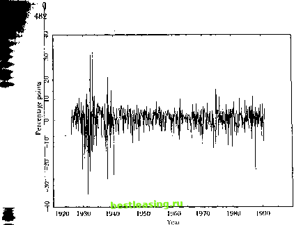 2000 Figure 12.2. Monthly Excess Log US Stock Hetums, 1926 to 1994 words, the volatility of asset returns appears to be serially correlated. This can be seen visually in Figure 12.2, which plots monthly excess returns on the CRSP value-weighted stock index over the period from 1926 to 1994. The individual monthly returns vary wildly, but they do so within a range which itself changes slowly over time. The range for returns is very wide in the 1930s, Tor example, and much narrower in the 1950s and 1960s. An alternative way to understand this is to calculate serial correlation coefficients for squared excess returns or absolute excess returns. At 0.23 and 0.21, respectively, the first-order serial correlation coefficients for these series are about twice as large as the first-order serial correlatioti coefficient for returns themselves, 0.11, and are highly statistically significant since the standard error under the null of no serial correlation is l/s/T = 0.036. The difference is even more dramatic in the average of the fust 12 autocorrelation coefficients: 0.20 for squared excess returns, 0.21 for absolute excess returns, and 0.02 for excess returns themselves. This reflects the fact that the autocorrelations of squared and absolute returns die out only very slowly. To capture the serial correlation of volatility, Englc (1982) proposed the class of Autoregressive Conditionally Heteroskedastic, or ARCH, mod- els. These write conditional variance as a distributed lag of past squared innovations: af = w-f- (Л).,?, (12.2.4) where a(L) is a polynomial in the lag operator. To keep the conditional variance positive, w and the coefficients in or(/.) must be nonnegative. As a way lo model persistent movements in volatility without estimating a very large number of coefficients in a high-order polynomial a(l), Bollerslev (1986) suggested the Generalized Autoregressive Conditionally Heteroskedastic, or GARCH, model: af = oj + fi(l.)af {+ot(L),if, (12.2.5) where 15(1.) is also a polynomial in the lag operator. Ну analogy with ARMA models, this is called a GARCH(/), ф model when the order of the polynomial P(l.) is /land the order of the polynomial a (I.) is </. The most commonly used model in the GARCH class is the simple GARCH(1,1) which can be written as a? = oj + fiaf l + an2 = oj+ (a -f/i)a2 , + a(i)2-of,) = ш + (a + fi)af , + aal,(cf - 1). (12.2.6) In the second equality in (12.2.6), the term (i]l-a2 ,) has mean zero, conditional on time ( - 1 information, and can be thought of as the shock to volatility. The coefficient a measures the extent to which a volatility shock today feeds through into next periods volatility, while (a-rfi) measures the rale at which this effect dies out over lime. The third equality in (12.2.6) rewrites the volatility shock as cr2 , (e2 - 1), the square of a standard normal less its mean-that is, a demeaned x2(I) random variable-multiplied by past volatility af {. The GARCH (1,1) model can also be written in terms of its implications for squared innovations n2+l. We have n2+, = > + ( + P) f + ilUt - ?) - Pili ~ o2 ,). (12.2.7) This representation makes it clear that the GARCII(1,1) model is an ARMA(I,1) model for squared innovations; but a standard ARMA(1,1) model has homoskedastic shocks, while here the shocks (;;2+ -af) are themselves heteroskedastic. Persistence and Slalionarily In the GARCH(1,1) model it is easy to construct multiperiod forecasts of volatility. When or 4- B<\, the unconditional variance of orcquivalendy the unconditional expectation olaf, is <o/( I - a-fi). Recursively suhsiittit- 1 2 3 4 5 6 7 8 9 10 11 12 13 14 15 16 17 18 19 20 21 22 23 24 25 26 27 28 29 30 31 32 33 34 35 36 37 38 39 40 41 42 43 44 45 46 47 48 49 50 51 52 53 54 55 56 57 58 59 60 61 62 63 64 65 66 67 68 69 70 71 72 73 74 75 76 77 78 79 80 [ 81 ] 82 83 84 85 86 87 88 89 90 91 92 93 94 95 96 97 98 99 100 101 102 103 |