l z. Nonlinearities in Financial Data

ing in (12.2.(i), and using ilu1 law of iterated expectations, die conditional expectation of volatility j periods ahead is

file iiiultipcrioti volatility forecast reverts lo its unconditional mean at rale (1* + p). This relation between single-period and multiperiod forecasts is the same as in a linear Л1ШЛ(1,1) model with autoregressive coefficient (a + p). Multiperiod forecasts can be constructed in a similar fashion for higher-order CARCI I models.

When a 4- /i= 1, the conditional expectation of volatility j periods ahead is instead

= f + jto. (12.2.9)

The GARCH (1,1) model with a + p = 1 has a unit autoregressive root so lhat todays volatility affects forecasts of volatility into the indefinite future. It is therefore known as an integrated CARCI1, or K.ARCl 1( 1,1), model.

The К IARCI1(1,1) process for oj looks very much like a linear random walk with drift w. 1 lowever Nelson (1990) shows that this analogy must be treated with caution. A linear random walk is nonsiationai у in two senses, first, il has no stationary distribution, hence the process is 1101 .strictly .stationary. Second, il has no unconditional first or second moments, hence it is not covariance stationary. In die I CARCI I( 1,1) model, on the other hand, of is strictly stationary even though its stationary distribution generally hicks unconditional moments. Thus the IGARO.l 1( 1,1) model is strictly stationary but not generally covariance stationary.

It is particularly easy to show dial the 1GARC11(1,1) model has ;> stationary distribution in the case where <u=0. Here (12.2.9) .simplifies to 1-К+(1=я, . so volatility is a martingale. At the same time, volatility remains bounded because it cannot go negative. Rut the martingale convergence theorem stales dial a hounded martingale must converge; in this case, the only value to which it can converge is /его. The stationary distribution for <7 - is then a degenerate distribution with point mass at /его, and this implies that the stationary distribution for iinl is also degenerate at /его. In this case the stationary distributions for a- and ; have moments, but they are all trivially /его.

When ii)>0, Nelson (1990) shows lhat there exists a nondegenerate stationary distribution for a,-. But this distribution does not have a finite mean or higher moments. The innovation r/,+i then has a stationary distribution with а /его mean, but with tails that are so thick that no second- or higher-order moments exist.

Nelson slums 1I1.1I these prnoci lies liolil more generally lor СЛК( !l l( 1,1} models with a + /I > 1 hut wiih l\lngt/t у (/<p (I.

12.2. Models of Changing Volatility 485

Alternative Functional Forms . ~>.....

In the standard GARCH model, forecasts of future variance are linear in current and past variances and squared returns drive revisions in the forecasts. An alternative model, sometimes known as the absolute value GARCH model, makes forecasts of future standard deviation linear in current and past standard deviations and has absolute values of returns driving revisions in the forecasts. An absolute value GARCH(1,1) model, for example, would be

cr, = oj +Pa,+aat-i\e,\. (12.2.10)

Schwert (1989) and Taylor (1986) estimate absolute value ARCH models, while Nelson and Foster (1994) discuss the absolute value GARCH(1,1).

The models we have considered so far are symmetric in that negative and positive shocks <?,+i have the same effect on volatility. However Black (1976) and many others have pointed out that there appears to be an asymmetry in stock market data: Negative innovations to stock returns tend to increase volatility more than positive innovations of the same magnitude. Possible explanations for this asymmetry are discussed in Section 12.2.3. To handle this, one can generalize the absolute value GARCH model to

cr, = oj + Po+ao.-ifie,), (12.2.11)

where

/( ,) = f, - 61 - c(6, - 6). (12.2.12)

Here the shift parameter b and the tilt parameter с measure two different types of asymmetry, b is unrestricted but we need c < 1 to ensure lhat /(*i)>0. When c=0 but 60, the effect of a shock on volatility depends on its distance from b, so that volatility increases more when there is no shock than when there is a shock of size b. When 6=0 but сфО, a zero shock has the .smallest impact on volatility but there is a distinction between positive and negative shocks; a shock of given size may have a larger effect whenj it is negative than when it is positive, or vice versa. Following Hentschel (1995), a nice way to understand (12.2.12) is to plot /(<=,) against e(, as in Figure 1.3.6 Panel (a) of the figure shows the absolute-value function (6=0, r=0); tlis is plotted again as a dashed line in each of the other panels. Panel (b) shows the shifted absolute-value function (6=0.5, c=0), panel (c) shows the tilted absolute-value function (6=0, c=0.25), and panel (d) shows a shifted and tilled absolute-value function (6=0.5, <= - 0.25).

Hentschel (1995) further generalizes (12.2.11) to allow a power of/(<?,), rather than /(<;,) itself, to affect volatility, and to allow a power of a rather

This is similar to the news impact curve of Pagan and Schwert (1990) and Engleland Ng (НШ), which plots af against holding any other relevant state variables at their unconditional means.

4&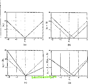

Figure 123. Shifted and Idled Absolute-Value Function

than a, itself, to be the variable that follows a linear difference equation. The resulting equation is

= OJ+в

(12.2.13)

Equation (12.2.13) defines a family of models lhat includes most of the popular GARCH-typc models in the literature.7 The standard GARCH model sets A=i>=2, and b=c=0. Glosten, Jagannathan, and Runkle (1993) have generalized the standard GARCH model to allow nonzero c. Engle and Ng (H 93) have instead allowed nonzero b. The absolute value GARCII model set:, A= =l with free ft and c. Another particularly important member of ihe fanjiily (12.2.12) is the exponential GARCH or EGARCH model of Nelson (1990), which is obtained by setting X=0, i>=1 , and /;=() to get

log(cr,) = со + /Hog(fj, i) + a [](,\ - ce,] .

Sec ;t l.sti Ding. Granger, and Knglc ( I.I.W) I с и ,t i elated I amity ot models.

(12.2.14)

This model is appealing because il does nol require any parameter restrictions to ensure that the conditional variance of the return is always positive. Also it becomes both strictly nonstationary and covariance nonstationary when a + fi=l, so it does not share the unusual statistical properties of the IGARCH(1,1) model. On the other hand, mulliperiod forecasts of future variances arc harder to calculate in the EGARCH model; no closed-form expressions like (12.2.8) are available.

Estimation

We have introduced an almost bewildering variety of volatility models. To discover which features of these models are important in lining financial data, one must be able to estimate the models parameters, fortunately this is fairly straightforward for GARCH models and other models in the class defined by (12.2.13). Conditional on the parameters of the model and an initial variance estimate, the data are normally distributed and wc can construct a likelihood function recursively. We write the vector of model parameters as (9, define о,(в) to be the conditional standard deviation at time . implied by the parameters and the history of returns, and define e,+ ](<9) s i),+i/o-,(0). When в contains the true parameters of the model, e,+ i(t9) is IID with density function g{el+i{в)) which we have assumed lo be standard normal:

= -L=r- <e)/:!. (12.2.15)

V27T

The conditional log likelihood of /,+ is therefore

г,(7/,+ 1;<9) = log(g( ;,+ i/ff,(e)))-log(c72(i9))/2 = -log(4/2lr )-+1/2r7,2(0)

-log(o,2(0))/2, (12.2.16)

where the last term is ajacobian term thai appears because we observe n,+ i and not ]/сг,(в). The log likelihood of the whole data set i/i.....n, is

С(щ.....nr) = ]Гс((и(+,;0). (12.2.17)

The maximum likelihood estimator is the choice ol parameters 0 that maximizes (12.2.17).

In practice one needs an initial a* to begin calculating the conditional likelihoods in (ГЛ2.lli). The influence olthe initial condition diminishes over time and becomes negligible asvmptoiic ally; thus the choice ol initial с onclifion does not alien the consistency ol the estimator.

/2. Nonlinearities in iinancial Data

Although it is easy lo show that the maximum likelihood estimator is consistent, it is harder to prove lhat il is asymptotically normal. The difficulty is that this requires regularity conditions which are hard to verily for CARCI I processes. I.ее and Hansen (1994) give some results for the CARCI 1(1,1) model Inn few other results tire available. F.mpirical researchers typicallv ignore this problem and assume that the usual regularity conditions hold. Some simulation evidence (Bollerslev and Wooldridgc 1992] and I.ums-daine 1995) supports this practice.

Hentschel (191)5) provides maximum likelihood estimates for a great variety of models in ihe family (I 2.2. IS) using daily and monthly stock relurn data over the period from 192(1 to 1990. To estimate the parameters X and i with any precision, Hentschel finds that he needs the very large number of observations provided by daily data. These daia suggest that X is close to one (as in the absolute value CARCI 1 model), but lhat i> is greater than one, in fact close lo 1.5. ln both daily and monthly data, Hentschel finds that asymmetry is belter modeled with the shift parameter I/ than with the lilt parameter c. Thus LIS stock returns are well-described by a GARCH model for the conditional standard deviation, driven by the shifted absolute value of shocks raised lo the power three halves. The volatility process is highly persistent in all the models estimated, although the degree of persistence is sensitive to specification in the post-World War II period.

Additional l\x/)ltintittii\ Variables

Dp lo ibis point we have modeled volatility using only the pasl history of returns themselves. Ii is straightforward to add other explanatory variables: For example, one can write an augmented CARCI 1(1,1) model as

nf = ш -)- у X, + /)rr,-. + a iff. (12.2.18)

where .V, is any variable known at time I. Provided that .\,>0 and y>0, this model still constrains volatility lo be positive. Alternatively, one can add explanatory variables lo ihe F.GARCI I model without any sign restrictions. Glosicii.Jagaiiiiailiaii.and Runkle (I99.i) add a short-term nominal interest rate to various GARCH models and show that il has a significant positive effect on stock market volatility.

Conditional Noil normality

The CARCI I models we have considered imply that the distribution of returns, conditional on the past history of returns, is normal. F.qtiivalenlly, the standardized residuals of these models, <=,и(0)=;;н /<т,(0), should be normal. Unfoi luualely, in practice there is excess kuriosis in the standardized residuals of GARCH models, albeit less than in the raw returns (see, for example, Bollerslev I987 and Nelson 1991 )).

12.2. Model, of Changing Volatility

One way lo handle this problem is to continue to work with the conditional normal likelihood function defined by (12.2.16) and (12.2.17)f but to interpret the estimator as a quasi-maximum likelihood estimator (White [1982]). Standard errors for parameter estimates can then be calculated using a robust covariance matrix estimator as discussed by Bollerslevand Wooldridge (1992).

Alternatively, one can explicitly model the fat-tailed distribution of the shocks driving a GARCH process. Bollerslev (1987), for example, suggests a Student-* distribution with к degrees of freedom:

(12.2.19)

where Г() is the gamma function. The t distribution converges to the normal distribution as к increases, but has excess kurtosis; indeed its fourth moment is infinite when к < 4. In a similar spirit Nelson (1991) uses a Generalized Error Distribution, while Engle and Gonzalez-Rivera (1991) estimate the error density nonparametrically.

GARCH models can also be estimated by Generalized Method of Moments (GMM). This is appealing when the conditional volatility of can be written as a fairly simple function of observed past variables (past squared returns and additional variables such as interest rates). Then the model implies that squared returns, less the appropriate function of the observed variables, are orthogonal to the observed variables. GMM estimation has the usual attraction that one need not specify a density for shocks to returns.

Stochastic-Volatility Models

Another response to the nonnormality of returns conditional upon past returns is to assume that there is a random variable conditional upon which returns are normal, but that this variable-which we may call stochastic volatility-is not directly observed. This kind of assumption is often made in continuous-time theoretical models, where asset prices follow diffusions with volatility parameters lhat also follow diffusions. Melino and Turnbull (1990) and Wiggins (1987) argue that discrete-time stochastic-volatility models are natural approximations to such processes. If we parametrize the discrete-time process for stochastic volatility, we then have a filtering problem: to process the observed data to estimate the parameters driving stochastic volatility and to estimate the level of volatility at each point in time.

A simple example of a stochastic-volatility model is the following:

i), = f ,r \ a, = фа, , 4- (12.2.20)

where c,~A/(0, af), £,~Л/ (0, er), and we assume lhat e, and £, are serially uncorrelated and independent of each other. Here a, measures the dif-