г./о 12. Nonliiienrities in Financial Data

H,b, and К11,11 I II, = H,B lo consinut a new error vector

vMl = (> , , -H,B ,)(H,B-y z.)

- (r , - II,B)(rM. , - H,b, )(H,b , - y ). (12.2.37)

I larvcv replaces e i in (12.2.3-1) \vi11i v, t t in (1 2.2.37), and drops the error мл i in (12.2.32). This gives a system with /. fewer orthogonality conditions and one less parameter to estimate (since Y\ drops out of lite model). The number of ovetidentifying restrictions declines by /. - I. Harvey (1989) finds some evidence that the price of risk varies when a US slock index is used as the market portfolio; however he also rejects the overidentifving restrictions of the model. Harvey (1991) uses a world stock index as the market portfolio and obtains similar results.

The Conditional CAIM and the Unconditional CAPM Equations (12.2.35) and (12.2.30) can be rewritten as

li n I H, = г + /Ы (12.2.38)

where /! = (a>\j/,. i. ,. i 11, / Y.n r, .,+1 H,l, the conditional beta ol asset iwith t he mat kel ret ш il, and Л, == 1>, .м1 I H,l- Kii.lhe expected excess leini n on the market over a riskless return.

aganualhan and Wang (1990) emphasize that this conditional version ol ihe CAIM need not imply the unconditional CAPM that was discussed in Chapter 5. If we lake unconditional expectations of (12.2.38), we get

K[r,Mtl = yi, + (E[/i i)(EX,l)+ Cov(/), A,). (12.2.39)

Here ЕЛ, is the unconditional expected excess return on the market. El/1 1 is the unconditional expectation of the conditional beta, which need not be the same as the unconditional beta, although the difference is likely lo be small. Most important, the covariance between the conditional beta and tin- expet ted excess market relurn A., appears in (12.2.39). Assets whose betas are high when the market risk premium is high will have higher unconditional mean returns than would be predicted by the unconditional (АРМ. Jagannathan and Wang (1990) argue that the high average returns on small stocks might be explained by this effect if small-stock betas tend lo rise al limes when the expected excess return on the slock market is high. They present some indirect evidence for this story although they do not directly model the time-variation of small-slock betas.

Volatility Innovations and Return Innovations

Empirical researcheis have found little evidence that periods of high volatility in slock reiuiiis are periods ol high expected stock returns. Some papers report weak evidence for this relationship (see Bollerslev, Engle, and

12.2. Models of Changing Volatility

Wooldridge [1988], French, Schwert, and Stambaugh [1987], and Harvey [ 1989]), but other papers which use the short-term nominal interest rate as an instrument find a negative relationship between the mean and volatility of returns (see Campbell [1987] and Glosten, Jagannathan, and Runkle [1993]).

As French, Schwert, and Stambaugh (1987) emphasize, there is much stronger evidence that positive innovations to volatility are correlated with negative innovations to returns. We have already discussed how asymmetric CARCI I models can fit this correlation. At a deeper level, it can be explained in one of two ways. One possibility is that negative shocks to returns drive up volatility. The leverage hypothesis, due originally to Black (1976), says that when the total value of a levered firm falls, the value of its equity becomes a smaller share of the total. Since equity bears the full risk of the firm, the percentage volatility of equity should rise. Even if a firm is not financially levered with debt, this may occur if the firm has fixed commitments to workers or suppliers. Although there is surely some truth to this story, it is hard to account for the magnitude of the return-volatility correlation using realistic leverage estimates (see Christie [1982] and Schwert [1989]).

An alternative explanation is that causality runs the other way: Positive shocks to volatility drive down returns. Campbell and Hentschel (1992) call this the volatility-feedback hypothesis. If expected stock returns increase when volatility increases, and if expected dividends are unchanged, then stock prices should fall when volatility increases. Campbell and Hentschel build this into a formal model by using the loglinear approximation for returns (7.2.26):

n+i = E,[r,+]] +4d,t+i -4 i+], (12.2.40)

where

f]d,l+\ = E,+ ]

is the change in expectations of future dividends in (7.2.25), and

4r,i+i = E,.

.>=>

E,

ХУг+1+;

is the change in expectations of future returns.

Campbell and Hentschel model the dividend news variable as

a GARCH(1,1) process with a zero mean: 4d,i+\~N(fl,o}), where of = ш 4- fiof ! 4- ai;*,.9 They model the expected return as linear in the variance

In fart ihcy use a more general asymmetric model, the quadratic GARCH or QCARCH model ol Seuiana (1991). This is to allow the model lo fil asymmetry in returns even in the absence of volatility feedback. However the basic idea is more simply illustrated using a standard CARCI I model.

of dividend news: E,[r,+ ]] = yo + Y\af. These assumptions imply dial the revision in expectations of all future returns is a multiple of todays volatility shock Ui

r.(+l

-<+l

X>Vt+i

(12.2.41)

where в=у\ра/(1-р(а + ji)). The coefficient 0 is large when y\ is large (for then expected relurns move strongly with volatility), when a is large (for then shocks feed strongly into future volatility), and when a 4- fi is large (for then volatility shocks have persistent effects on expected returns). Substituting into (12.2.40), the implied process for returns is

r,+ i = Ко + Y\o} + n,/ + i - i - of)-

(12.2.42)

This is .not a GARCH process, but a quadratic function of a GAKCII process. It implies that returns are negatively skewed because a large negative realization of will be amplified by the quadratic term whereas a large positive realization will be damped by the quadratic term. The intuition is that any large shock of either sign raises expected future volatility and required returns, driving down the slock return today. Conversely, no news is good news ; if n<u-H=0 this lowers expected future volatility and raises the stock return today. Campbell and Hentschel find much stronger evidence for a [positive price of risk y\ when they estimate the model (12.2.42) than when (they simply estimate a standard GARCf I-M model. Their results suggest that Iboth the volatility feedback effect and the leverage effect contribute to the asymmetric behavior of slock market volatility.

12.3 Nonparametric Estimation

In some financial applications we may be led to a functional relation between two variables Y and X without the benefit of a.structural model to restrict the parametric form of the relation. In these situations, we can use nonparametric estimation techniques to capture a wide variety of nonlinearilies without recourse to any one particular specification of the nonlinear relation. In contrast to the relatively highly structured or parametric approach to estimating nonlinearilies described in Sections 12.1 and 12.2, nonparametric estimation requires few assumptions about the nature of the nonlinearilies. However, this is not without cost-nonparametric estimation is highly data-intensive and is generally not effective for smaller sample sizes. Moreover, nonparametric estimation is especially prone to overfilling, a problem lhat cannot be easily overcome by statistical methods (sec Section 12.5 below).

Perhaps the most commonly used nonparauictric estimators arc smoothing estimators, in which observational errors are reduced by averaging the data in sophisticated ways. Kernel regression, orthogonal series expansion, projection pursuit, nearest-neighbor estimators, average derivative estimators, splines, and artificial neural networks are all examples of smoothing. To understand the motivation Tor such averaging, suppose that we wish lo estimate the relation between two variables Г, and X, which satisfy

Y, = w(X,) + f I = 1.....7, (12.3.1)

where mi) is an arbitrary fixed but unknown nonlinear function and {(,) is a zero-mean IID process.

Consider estimating m() at a particular dale t{, for which X=x , and suppose that lor this one observation X, , we can obtain repealed independent observations of the variable Yk say Y=y\,.... F, =V Then a natural estimator of the function w(-) al the point is

1 1

т(*ъ) = - Y yi = - V* [ , (*,) + J ] (12.3.2)

1

= mU) 4-- (12.3.3)

and by die Law of Large Numbers, the second term in (12.3.3) becomes negligible for large n.

Of course, if j Yt\ is a time series, we do not have the luxury of repeated observations for a given X,. However, if we assume that the function m(-) is sufficiently smooth, then for time-series observations X, near the value x , the corresponding values of Y, should be close to m(xo). In other words, if ( ) is sufficiently smooth, then in a small neighborhood around xo, m(xo) will be nearly constant and may be estimated by taking an average of ihe K,s that correspond lo those X/s near xn. The closer the X,s are to the value xa, the closer an average of corresponding f ,s will be to ?и(д). This argues for a weighted average of the У/s, where the weights decline as the X,s get farther away from *<> This weighted average procedure оГ estimating m(x) is the essence of smoothing. More formally, for any arbitrary x, a smoothing estimator of m(x) may be expressed as

mix) = -\<ouix)Y,. (12.3.4)

where the weights oi,.y (x)) are large for those ),s paired with X,s near and small for those K,s with X,s far from x.

To implement such a procedure, we must define what we mean by near and far . If we choose too large a neighborhood around x to compute the

average, the weighted average will he loo smooth and will not exhibit the genuine nonlinearities ol wi(). If we choose too small a neighborhood around ,v, (he weighted average will he too variable, reflecting noise as well as the variations in / ( ). Therefore, the weights ((i>( ,;(x)! must he chosen carcltilly lo balance ihese two considerations. We shall address this and other related issues explicitly in Sections 12.3.1 to 12.3.3 and Section 12.Г).

12.3.1 Kernel Regression

An important smoothing technique for estimating w() is kernel regression. In the kernel regression model, the weight function ш, j\x) is constructed from a probability density function K(.v), also called a kernel:

K(x) > (I, j K(u)<t = 1. (12.3.5)

Despite the fact thai K(.v) is a probability density function, il plays no probabilistic role in the subsequent analysis-it is merely a convenient method for computing ;i weighted average, and does not imply, for example, that X is distributed according to K(x) (which would be a parametric assumption).

By rcsealing the kernel with respect to a variable /<>(), we can change its spread by varying Ii if we define:

k ( ) = j-K( ;), j Ki,{u)du = 1. (12.3.(i)

Now we can define the weight function to be used in the weighted average (12.3.4) as

to r{x) == K;,(x- X,)/g (x) (li.3.7)

g (x) = -]Гк (х-X,). (12.3.8)

If It is very small, the averaging will he done with respect lo a rather small neighborhood around each of die A,s. If h is very large, the averaging will be over larger neighborhoods of the .V,s. Therefore, controlling the degree of averaging amounts to adjusting the smoothing parameter Л, also known as the Ixmdwiillh} Substituting (12.3.8) into (12.3.4) yields the Nadaraya-Witlson kernel estimator w/,(x) of wfx):

I \A У\ K/i(* - Л,) 1,

/,<v) = -V(,v/(,v)i; = --. (12.3.!))

i tr L,=iM*-.v()

Clioiisinr; Ни- ;ii(in>ii iair luuilwiilili is discussed inure fully in Serlion 12.1.2.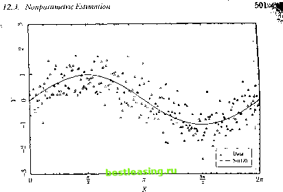

Figure 12.4. Simulation of Y, = Sin(X,) + 0.5*,

Under certain regularity conditions on the shape of the kernel К and the magnitudes and behavior of the weights as the sample size grows, it may be shown that m/,(x) converges to m(x) asymptotically in several ways (see Hurdle [1990] for further details). This convergence property holds for a wide class of kernels, but for the remainder of this chapter and in our empirical examples we shall use the most popular choice of kernel, the Gaussian kernel:

K (x) = -==е~. (12.3.10)

h-j2n

An Illustration of Kernel Regression

To illustrate the power of kernel regression in capturing nonlinear relations, we apply this smoothing technique to an artificial dataset constructed by Monte Carlo simulation. Denote by (X,) a sequence of 500 observations which take on values between 0 and 2л at evenly spaced increments, and lei I),) be related to (X,) through the following nonlinear relation:

Y, = Sin(X,) 4-0.5f, (12.3.11)

where {f,} is a sequence of IID pseudorandom standard normal variates. Using the simulated data (X Y,\ (see Figure 12.4), we shall attempt to estimate the conditional expectation E[ Y, X,] = Sin(X,), using kernel